An R package confusionMatrices enables plotting confusion matrices, highlighting their main and parallel diagonals, and calculating performance metrics.
library(devtools)
devtools::install_github("LStepanek/confusionMatrices")

library(confusionMatrices)
Below are several examples that demonstrate the usage of the plotConfusionMatrix() function. Each example progressively introduces more complexity and highlights different features of the function.
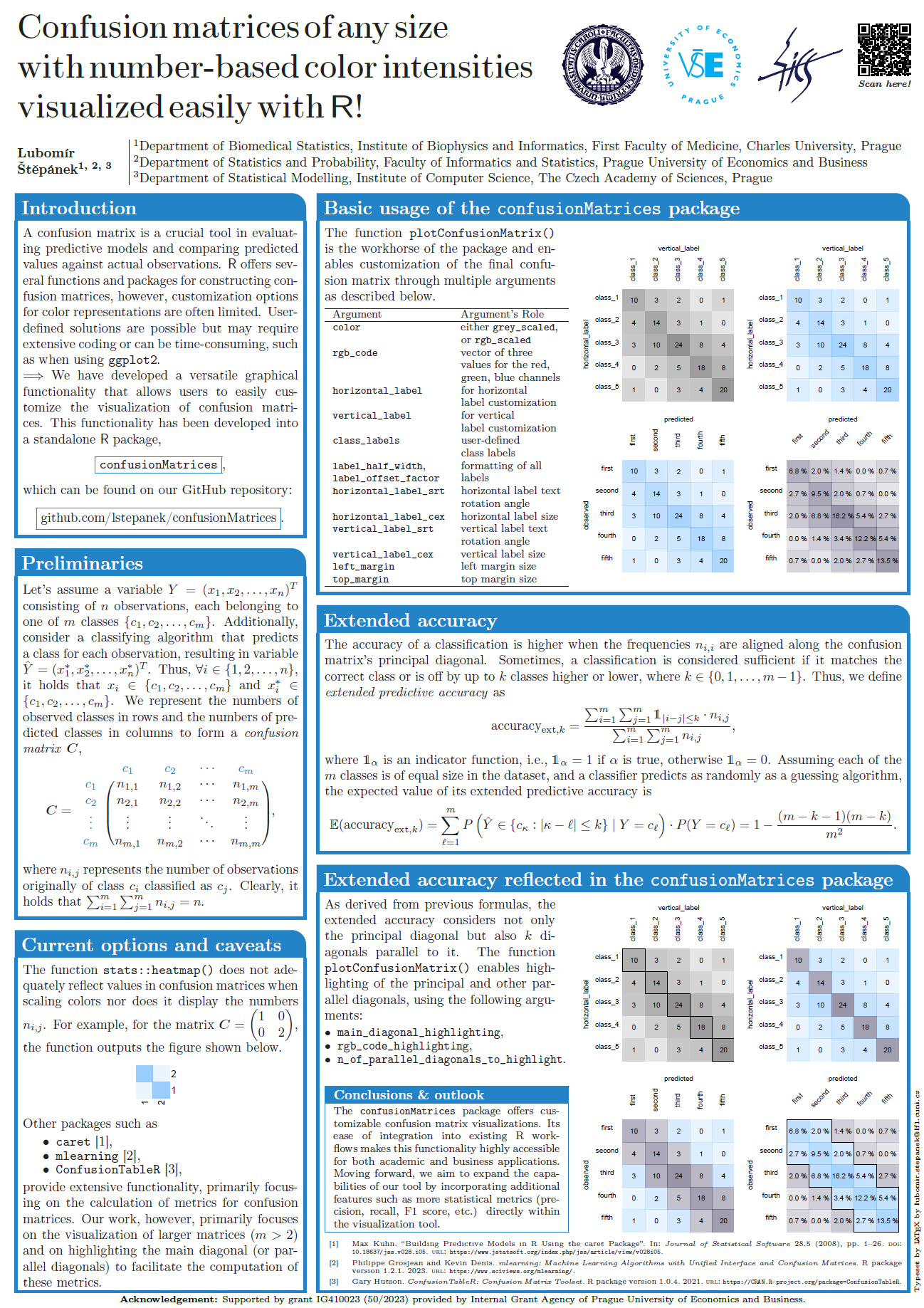
This simple example demonstrates the default usage of the function with a basic confusion matrix, utilizing default color scaling and no highlighting.
# Define a basic confusion matrix
basic_table <- matrix(
    c(10, 2, 3, 0,
      0, 15, 0, 1,
      0, 1, 20, 2,
      1, 0, 3, 18),
    nrow = 4,
    byrow = TRUE,
    dimnames = list(
        observed = c("class_1", "class_2", "class_3", "class_4"),
        predicted = c("class_1", "class_2", "class_3", "class_4")
    )
)

# Plot the basic confusion matrix
plotConfusionMatrix(
    table = basic_table,
    color = "grey_scaled",
    main_diagonal_highlighting = "none",
    percentage_display = FALSE
)
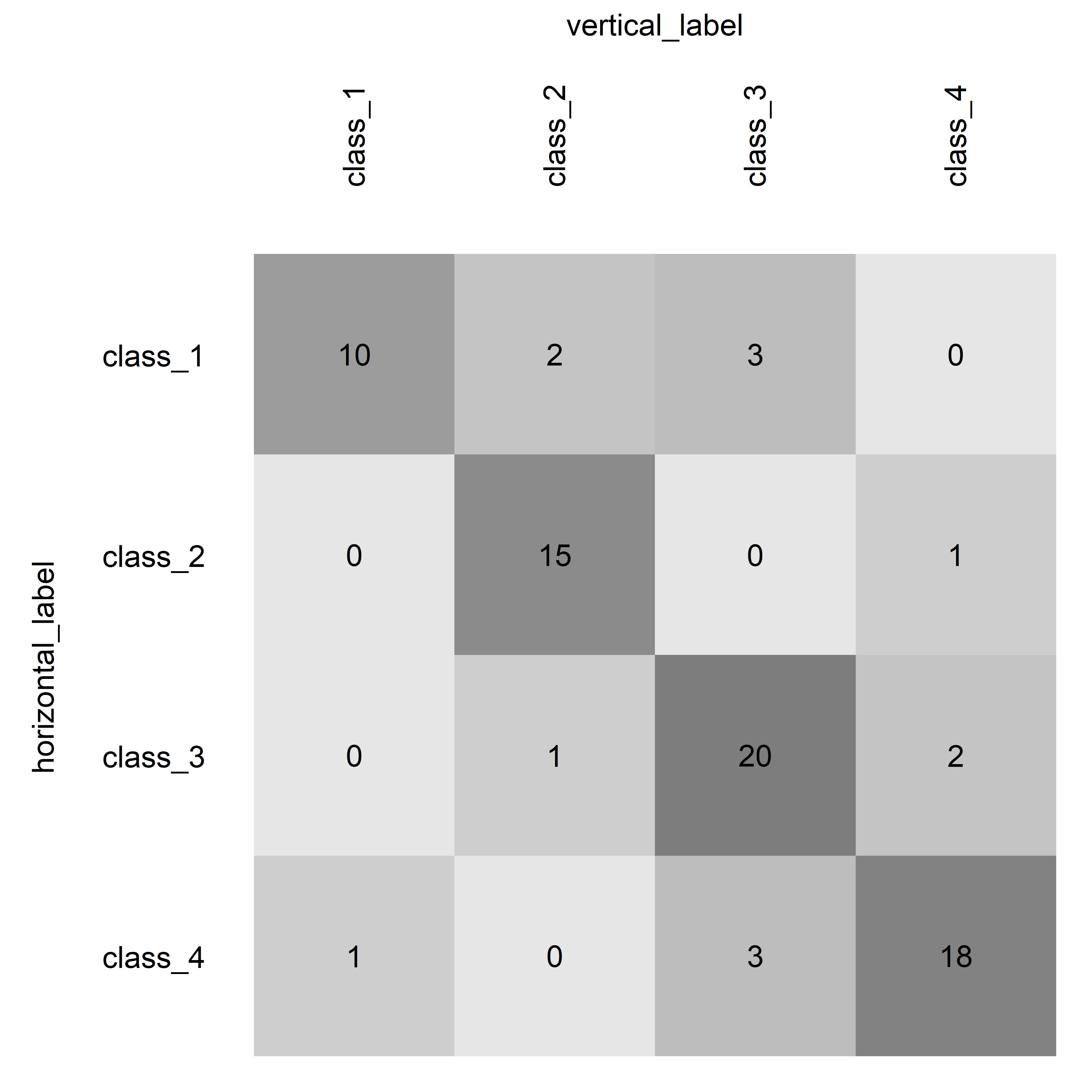
This example uses RGB color scaling and adds custom labels to the axes, making it slightly more complex and visually distinct.
plotConfusionMatrix(
    table = basic_table,
    color = "rgb_scaled",
    rgb_code = c(0.2, 0.5, 0.7),
    horizontal_label = "Actual Classes",
    vertical_label =  "Predicted Classes",
    main_diagonal_highlighting = "none",
    percentage_display = FALSE
)
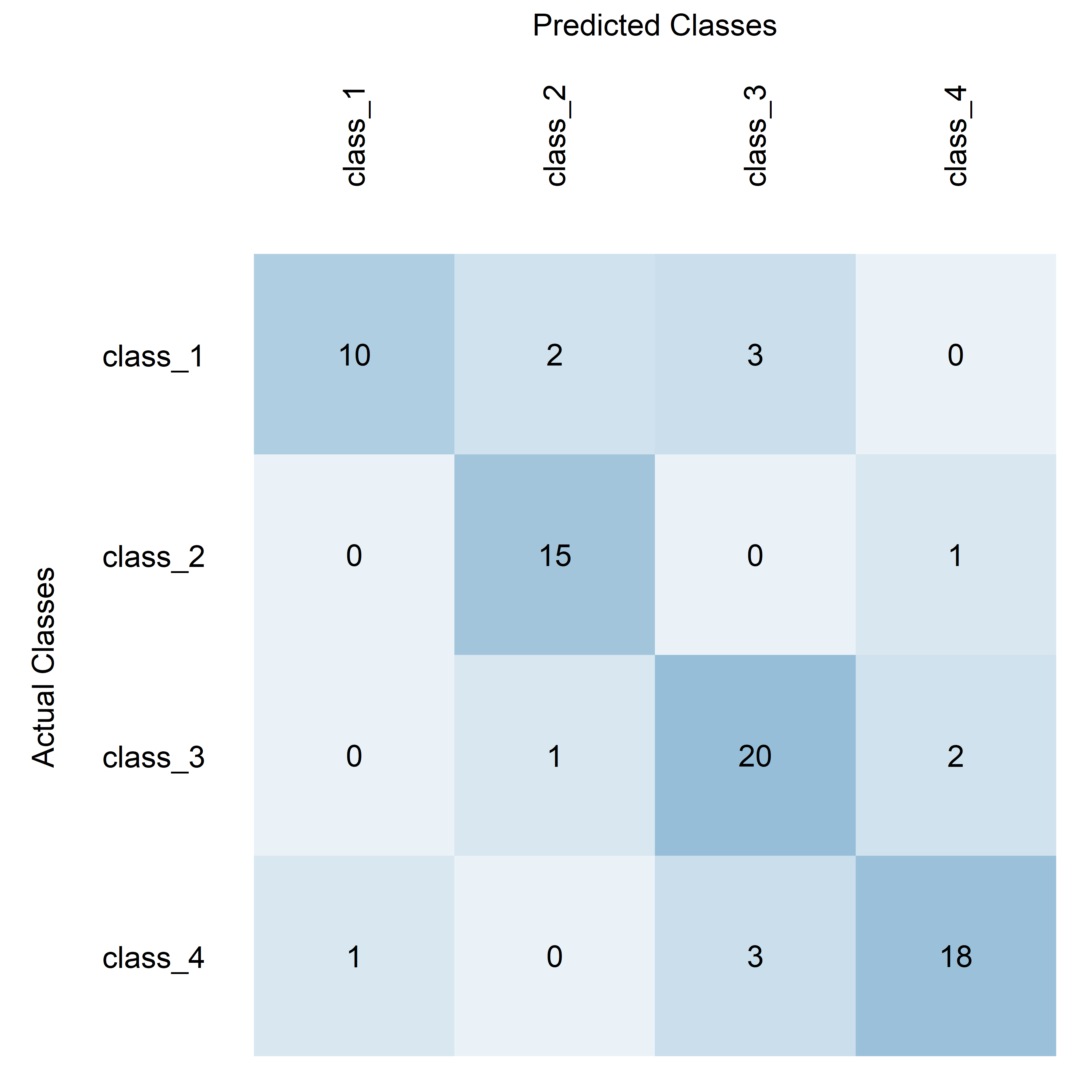
This example introduces diagonal highlighting and custom class labels, showcasing the function's capability to emphasize specific parts of the matrix and label classes differently.
plotConfusionMatrix(
    table = basic_table,
    color = "rgb_scaled",
    rgb_code = c(0.6, 0.1, 0.1),
    class_labels = c("Type 1", "Type 2", "Type 3", "Type 4"),
    main_diagonal_highlighting = "color",
    rgb_code_highlighting = c(1, 0, 0),
    percentage_display = FALSE
)
This final example uses a comprehensive set of customizations, including highlighting multiple diagonals, displaying percentages, and adjusting text and frame properties, representing the most complex use case.
# Define a larger, more complex confusion matrix
complex_table <- matrix(
    c(30, 5, 2, 1, 0,
      3, 40, 0, 2, 1,
      0, 2, 50, 3, 2,
      1, 0, 4, 45, 5,
      0, 1, 2, 5, 35),
    nrow = 5,
    byrow = TRUE,
    dimnames = list(
        observed = c("class_A", "class_B", "class_C", "class_D", "class_E"),
        predicted = c("class_A", "class_B", "class_C", "class_D", "class_E")
    )
)

# Plot the complex matrix with extensive customizations
plotConfusionMatrix(
    table = complex_table,
    color = "rgb_scaled",
    rgb_code = c(0, 0.4, 0.8),
    class_labels = c("Alpha", "Beta", "Gamma", "Delta", "Epsilon"),
    main_diagonal_highlighting = "both",
    rgb_code_highlighting = c(0.8, 0.2, 0.2),
    rgb_code_highlighting_framebox = c(0, 0, 0),
    highlighting_framebox_lwd = 2.0,
    n_of_parallel_diagonals_to_highlight = 1,
    percentage_display = TRUE,
    percentage_round_digits = 2,
    horizontal_label = "True Category",
    vertical_label = "Predicted Category",
    horizontal_label_cex = 0.8,
    vertical_label_cex = 0.8,
    left_margin = 6.0,
    top_margin = 6.0
)
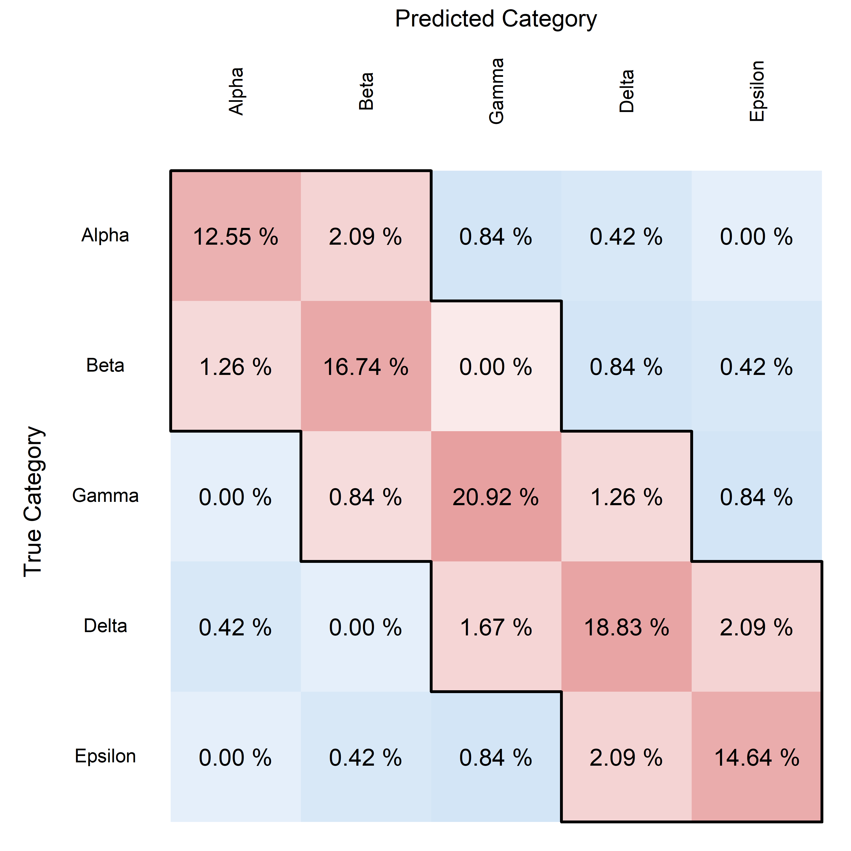
These examples start from very basic usage and move towards increasingly complex scenarios, demonstrating the flexibility and powerful visualization capabilities of the plotConfusionMatrix function.
The function getAccuracy provides a versatile way to calculate the accuracy of a classification model based on the alignment along the diagonal(s) of a confusion matrix. Below are examples demonstrating how to use this function with different settings for the n_of_parallel_diagonals_to_consider parameter. The examples assume complex_table is a predefined confusion matrix available within the package.
This example calculates traditional accuracy, considering only exact matches between the predicted and actual classes. This is the strictest measure of accuracy, focusing solely on perfect predictions.
getAccuracy(
    table = complex_table,
    n_of_parallel_diagonals_to_consider = 0
)
> $accuracy
> [1] 0.8368201
>
> $expected_accuracy
> [1] 0.2
This example extends the concept of accuracy to include predictions that are off by one class. It considers predictions that are either one class higher or one class lower than the actual class as correct. This approach is particularly useful in ordered classes where adjacent categories may carry similar practical implications.
getAccuracy(
    table = complex_table,
    n_of_parallel_diagonals_to_consider = 1
)
> $accuracy
> [1] 0.9497908
>
> $expected_accuracy
> [1] 0.52
The getAccuracy function's flexibility allows users to define what constitutes an accurate prediction, making it adaptable to various practical scenarios. By adjusting the n_of_parallel_diagonals_to_consider, users can tailor the strictness of the accuracy calculation to reflect realistic expectations and the nature of the classification task at hand. The comparison between the calculated $accuracy and the $expected_accuracy of a random classifier is crucial for assessing the true effectiveness of our model. It helps in understanding whether the improvements in accuracy are due to the model's predictive capabilities or merely due to chance. This comparison also provides a baseline to gauge the performance enhancements needed and helps in making informed decisions about further model development and deployment strategies.
Poster from useR!2024 Conference