KronosTheLate / EasyFFTs.jl

An opinionated layer on top of FFTW.jl to provide simpler FFTs for everyone.

EasyFFTs

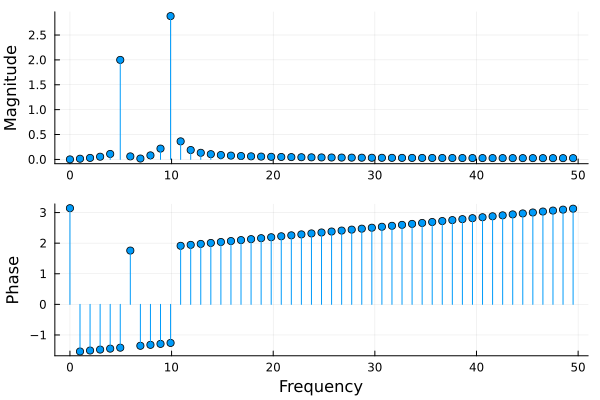
Are you sick and tired of always doing the same preprocessing before you can visualize your fft? Look no further. EasyFFTs aims to automate common preprocessing of fft's, aimed at visual inspection of the frequency spectrum. The main workhorse of this package is a very simple function easyfft that modifies the output of fft and rfft from FFTW.jl slightly.

This function offers four main benefits to using the FFTW functions directly:

• The output is scaled by default, making the absolute value of the response correspond directly to the amplitude of the sinusoids that make up the signal.
• Simple and short syntax for getting the associated frequencies from sample frequency.
• Frequencies and response are sorted by increasing frequency (if you have ever used fftshift you know what I am talking about)
• rfft is automatically called for real input signals, avoiding the common mistake of always using fft. This makes it so that half of the symmetric spectrum is not computed, and not returned. This reduces computation and allocations, without loss of information. If you want both sides of the spectrum, use easymirror, with usage demonstrated in the docstring.

In case you also want to compute the "as the mathematicians define it" Discrete Fourier Transform, this package reexports everything exported from FFTW, so that using EasyFFTs; fft(rand(100)) is equivalent to using FFTW; fft(rand(100)). The only difference between using EasyFFTs and using FFTW is therefore that EasyFFTs exports a few extra functions that mainly facilitate visualization of the spectrum.

Examples

It is easier to explain by example, so view the examples below as a light introduction to all function defined in EasyFFTs, and how to use them.

Setup

First, we need something to analyze. Let's define some sample-timestamps:

julia> using EasyFFTs

julia> fs = 100;  # sampling frequency

julia> timestamps = range(0, 1, step = 1 / fs);  # One second signal duration

We then make a signal s composed of 2 pure sinusoids with frequencies of 5 Hz and 10 Hz, sampled at timestamps:

julia> f1 = 5 ; A1 = 2;

julia> f2 = 10; A2 = 3;

julia> s = @. A1 * sin(f1 * 2π * timestamps) + A2 * sin(f2 * 2π * timestamps);

How to use easyfft

Lets now use easyfft, and bind the output to ef:

julia> ef = easyfft(s, fs)
EasyFFT with 51 samples.
Dominant component(s):                  
   Frequency  │  Magnitude   
╺━━━━━━━━━━━━━┿━━━━━━━━━━━━━╸
     9.901    │   2.8796     
╶─────────────┼─────────────╴
    4.9505    │   1.9997     

The output is of the type EasyFFT, so to understand the output (bound to ef), we have to understand the type. It is not complicated at all. In fact, it essentially acts as a NamedTuple. The reason for wrapping the output in a new type is the pretty printing seen above, and automatic plotting. Note that the pretty printing rounds values to 5 significant digits.

The EasyFFT type

The type EasyFFT contains frequencies and the corresponding (complex) responses. There are 3 different ways to access the frequencies and responses, just like for named tuples. The first is way "dot syntax":

 julia> ef.freq
51-element Vector{Float64}:
  0.0
  0.9900990099009901
  ⋮
 48.51485148514851
 49.504950495049506

 julia> ef.resp
51-element Vector{ComplexF64}:
 -9.578394722256253e-17 + 0.0im
 0.00042622566734221867 - 0.013698436692159435im
                        ⋮
  -0.025328817492520122 + 0.0011826329422999651im
   -0.02532460367843232 + 0.00039389110927144075im

Should you ever forget that you should use freq and resp, the Base Julia function propertynames will remind you.

julia> propertynames(ef)
(:freq, :resp)

The second method is iteration, which allows for destructuring assignment into seperate variables:

julia> frequencies, response = easyfft(s, fs);

julia> ef.freq == frequencies
true

julia> ef.resp == response
true

The third and final way of accessing the frequencies and response is indexing:

julia> ef.freq == frequencies == ef[1]
true

julia> ef.resp == response == ef[2]
true

Convenience functions

Convenience functions are defined to extract the magnitude and phase of the response:

julia> magnitude(ef) == abs.(ef.resp)
true

julia> phase(ef) == angle.(ef.resp)
true

Appending a d to phase will get you the angle in degrees, analogous to sin and sind:

julia> phased(ef) == rad2deg.(phase(ef))
true

We saw that objects of the type EasyFFT are displayed as a table of the dominant frequencies. The functions used to find the dominant values are exported.

We can get the dominant frequencies like so:

julia> domfreq(ef)
2-element Vector{Float64}:
 9.900990099009901
 4.9504950495049505

And their indices like so:

julia> finddomfreq(ef)
2-element Vector{Int64}:
 11
  6

Sometimes we want to know the response at a specific frequency. This functionality is provided by the response_at function:

julia> response_at(ef, 5)
(freq = 4.9504950495049505, resp = 0.3097558587965989 - 1.9756025627302725im)

julia> response_at(ef, [5, 10])
(freq = [4.9504950495049505, 9.900990099009901], resp = ComplexF64[0.3097558587965989 - 1.9756025627302725im, 0.881335139504854 - 2.741456352889268im])

Finally, you can get the symmetric spectrum using easymirror:

julia> easymirror(ef)
EasyFFT with 101 samples.
Dominant component(s):                   
   Frequency  │  Magnitude   
╺━━━━━━━━━━━━━┿━━━━━━━━━━━━━╸
    -9.901    │   1.4398     
╶─────────────┼─────────────╴
     9.901    │   1.4398     
╶─────────────┼─────────────╴
    -4.9505   │   0.99987    
╶─────────────┼─────────────╴
    4.9505    │   0.99987    

The amplitudes are adjusted correctly, halving the magnitude of all component except for the 0 Hz component.

That wraps up the examples for the functions defined in EasyFFTs. Each function has a docstring with a lot more detail about the method signatures and arguments, so check that out if if you have questions. If anything is still unclear, please open up an issue.

Plotting

Because the returned value is of a custom type, automatic plot recipes can be defined. This has been done for Plots.jl:

using Plots
plot(ef)

For less than 100 datapoints, the plot defaults to a stem plot, which is the most appropriate for showing discrete quantities. However, stem plots get messy and slow with too many points, which is why the default changes to a line plot if there are 100 datapoints or more. Change the keywords seriestype and markershape in the call to plot to customize the behavior.