tsfeatures

The R package tsfeatures provides methods for extracting various features from time series data.

Installation

The stable version on R CRAN is coming soon.

You can install the development version from Github with:

# install.packages("devtools")
devtools::install_github("robjhyndman/tsfeatures")

Usage

Hyndman, Wang and Laptev (ICDM 2015)

library(tsfeatures)
library(tidyverse)
library(anomalous)

# Compute the features used in Hyndman, Wang & Laptev (ICDM 2015).
# Note that crossing_points, peak and trough are defined differently 
# in the tsfeatures package than in the Hyndman et al (2015) paper. 
# Other features are the same. Using the real data from the paper
yahoo <- cbind(dat0, dat1, dat2, dat3)
hwl <- bind_cols(
         tsfeatures(yahoo,
           c("acf_features","entropy","lumpiness",
             "flat_spots","crossing_points")),
         tsfeatures(yahoo,"stl_features", s.window='periodic', robust=TRUE),
         tsfeatures(yahoo, "max_kl_shift", width=48),
         tsfeatures(yahoo,
           c("mean","var"), scale=FALSE, na.rm=TRUE),
         tsfeatures(yahoo,
           c("max_level_shift","max_var_shift"), trim=TRUE)) %>%
  select(mean, var, x_acf1, trend, linearity, curvature, 
         seasonal_strength, peak, trough,
         entropy, lumpiness, spike, max_level_shift, max_var_shift, flat_spots,
         crossing_points, max_kl_shift, time_kl_shift)

# 2-d Feature space
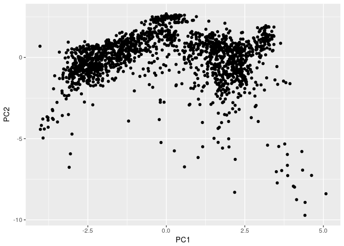
prcomp(na.omit(hwl), scale=TRUE)$x %>% 
  as_tibble() %>%
  ggplot(aes(x=PC1, y=PC2)) +
    geom_point()

Kang, Hyndman & Smith-Miles (IJF 2017)

library(tsfeatures)
library(tidyverse)
library(forecast)


# Compute the features used in Kang, Hyndman & Smith-Miles (IJF 2017).
# Note that the trend and ACF1 are computed differently for non-seasonal
# data in the tsfeatures package than in the Kang et al (2017). 
# tsfeatures uses mstl() which uses supsmu() for the trend calculation with 
# non-seasonal data, whereas Kang et al used a penalized regression spline
# computed using mgcv instead.  Other features are the same.

M3data <- purrr::map(Mcomp::M3, 
  function(x){
      tspx <- tsp(x$x)
      ts(c(x$x,x$xx), start=tspx[1], frequency=tspx[3])
  })
khs_stl <- function(x,...)
{
  lambda <- BoxCox.lambda(x, lower=0, upper=1, method='loglik')
  y <- BoxCox(x, lambda)
  c(stl_features(y,s.window='periodic', robust=TRUE, ...), lambda=lambda)
}
khs <- bind_cols(
  tsfeatures(M3data, c("frequency", "entropy")),
  tsfeatures(M3data, "khs_stl", scale=FALSE)) %>% 
  select(frequency, entropy, trend, seasonal_strength, e_acf1, lambda) %>%
  replace_na(list(seasonal_strength=0)) %>%
  rename(
    Frequency = frequency,
    Entropy = entropy,
    Trend = trend,
    Season = seasonal_strength,
    ACF1 = e_acf1,
    Lambda = lambda) %>%
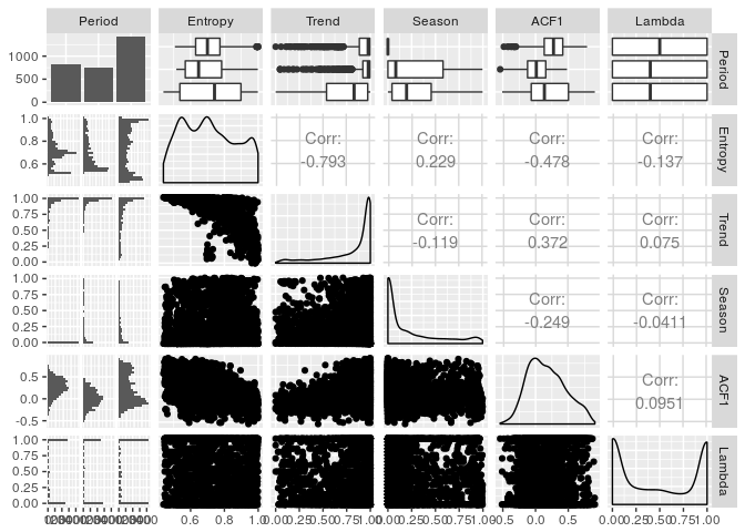
  mutate(Period = as.factor(Frequency))

# Fig 1 of paper
khs %>% 
  select(Period, Entropy, Trend, Season, ACF1, Lambda) %>%
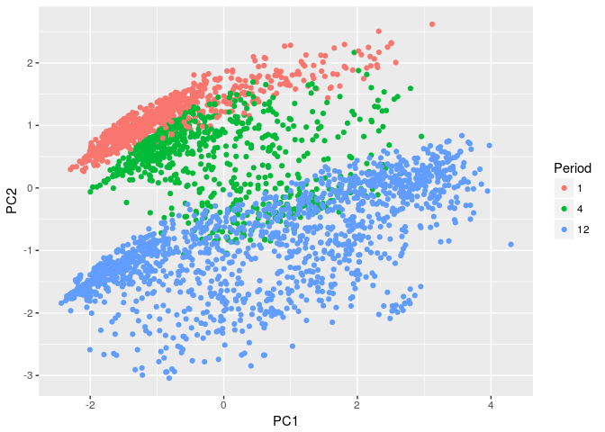
  GGally::ggpairs()

# 2-d Feature space (Top of Fig 2)
prcomp(select(khs, -Period), scale=TRUE)$x %>%
  as_tibble() %>%
  bind_cols(Period=khs$Period) %>%
  ggplot(aes(x=PC1, y=PC2)) +
    geom_point(aes(col=Period))

License

This package is free and open source software, licensed under GPL-3.

KathyGCY / tsfeatures