This is an R package providing some styling resources for web content intended to align with the graphical profile used at KTH Royal Institute of Technology.
It is heavily inspired by https://github.com/hrbrmstr/hrbrthemes. Most of the graphical design considerations, the package structure used and the functions are either ripped directly or modified slightly from that package. The styling assets and resources are different, though (fonts, templates, color palettes etc) and adapted to KTH’s graphical profile
It includes fonts in the two main font families used in the graphical profile of KTH:
- Figtree (SIL-licensed font)
- Open Sans (used to be the primary font; to be used for web content and for text inside plots)
- Open Sans Condensed is a narrow variant of Open Sans (looks even better in plots)
- Georgia (KTH has a license to use this MS font)
Two templates are provided for styling rmarkdown authored content:
- one for general HTML content with the KTH CSS styles
- one for PDF output
It also provides a theme_kth_neo() function which can be used to style
ggplots.
You can install the development version of ktheme from
GitHub with:
# install.packages("devtools")
devtools::install_github("KTH-Library/ktheme")A helper function is available for system-wide install of fonts on Linux OSes:
# install from https://github.com/KTH-Library/bibliomatrix
library(ktheme)
if(Sys.info()["sysname"] == "Linux")
  install_fonts_linux()

#library(extrafont)
#extrafont::loadfonts()

# required in the following usage examples
library(dplyr)
library(ggplot2)
library(Cairo)Three color palettes are provided; the new standard “kth_palette_neo()”, the previous standard “kth_palette()” and the previous “kth_palette_digital()” palette.
Palettes take their starting point in a set of colors used (at different points in time), currently originating from the KTH signature colors.
These color palette can be used to color qualitative data, sequential data and diverging data.
- qualitative palette for use with nominal or unordered categorical values (using the primary KTH profile color (blue), followed by profile colors, each color available in triplets (darker tone, lighter tone, medium tone), thus providing a total of 6 x 3 = 18 colors)
- sequential palette for quantitative magnitudes - high/low values - or for ordered categorical data (the “kth_palette” variant uses the primary color in 5 stepped variations - from the strongest tone stepping towards a neutral gray)
- diverging palette for use with quantitative values centered around some point - or centered ordered categorical data of that same nature (the primary color is used on one end of the palette and the closest complement color on the other to provide a 7-color palette with three steps of blue towards a gray midpoint and three steps of red away from that midpoint)
This palette is based on the standard KTH colors.
# for nominal categorical coloring, try to use five colors
palette_kth_neo(n = 6) %>% unname %>% show_pal()
# if you need to color more categorical data, use color pairs
palette_kth_neo(n = 12) %>% unname %>% show_pal(nrow = 2, ncol = 6)# for categorial colors there is a maximum of 15 color triplets
# use with caution as the medium and strong triplet members might be hard to distinguish
palette_kth_neo(n = 18) %>% unname %>% show_pal(ncol = 6, nrow = 3)# sequential categorical offers a maximum of 5 steps (primary color, fading towards gray)
palette_kth_neo(n = 5, type = "seq") %>% unname %>% show_pal()palette_kth_neo(n = 5, type = "seq") %>% unname %>% show_pal(borders = FALSE, labels = FALSE)# diverging categorical offers a maximum of 7 steps (primary color and complementary color, steps towards gray in the middle)
palette_kth_neo(n = 7, type = "div") %>% unname %>% show_pal()palette_kth_neo(n = 7, type = "div") %>% unname %>% show_pal(labels = FALSE, borders = FALSE)This palette is based on the previous set of KTH colors for Digital media
# all 5 colors (primary and secondary signature colors) in triplets (faded towards gray, "strong", "light" and "medium")
palette_kth_digital(n = 15) %>% unname %>% show_pal(nrow = 5, ncol = 3)
# sequential 5 steps (primary color, fading towards gray)
palette_kth_digital(n = 5, type = "seq") %>% unname %>% show_pal()# diverging 7 steps (primary color and complementary color, steps towards gray in the middle)
palette_kth_digital(n = 7, type = "div") %>% unname %>% show_pal(labels = FALSE, borders = FALSE)Here are usage examples showing (gg)plots made using the different KTH colour palettes with the Figtree font.
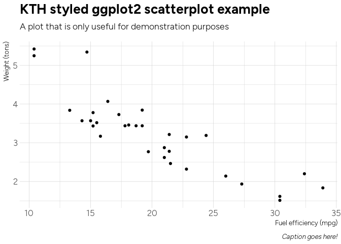
A plain vanilla scatter plot:
ggplot(mtcars, aes(mpg, wt)) +
  geom_point() +
  labs(x="Fuel efficiency (mpg)", y="Weight (tons)",
    title="KTH styled ggplot2 scatterplot example",
    subtitle="A plot that is only useful for demonstration purposes",
    caption="Caption goes here!") +
  theme_kth_neo()
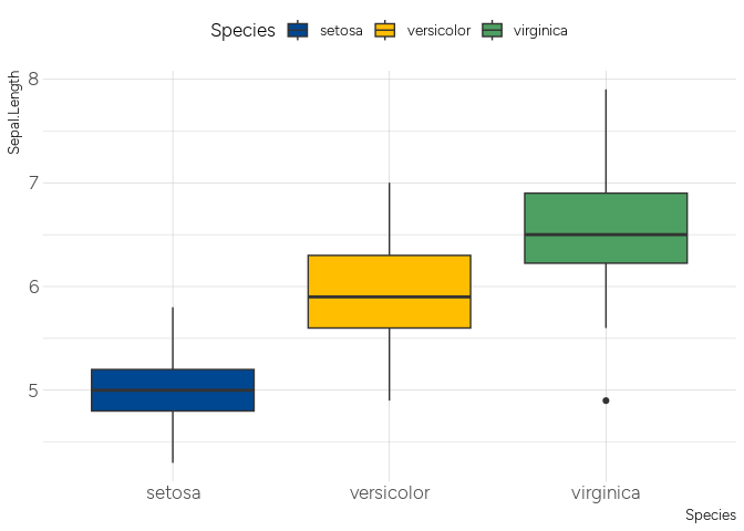
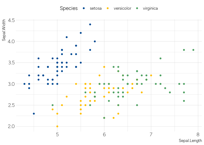
Using the KTH palette, qualitative coloring:
ggplot(iris, aes(Species, Sepal.Length)) +
  geom_boxplot(aes(fill = Species)) +
  scale_fill_kth() +
  theme_kth_neo() +
theme(legend.position = "top")ggplot(iris, aes(Sepal.Length, Sepal.Width)) +
geom_point(aes(color = Species)) +
scale_color_kth() +
theme_kth_neo() +
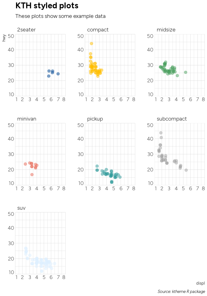
theme(legend.position = "top")Another example using demo data:
gg <-
  ggplot(mpg, aes(displ, hwy)) +
  geom_jitter(aes(color=class, fill=class), size=3, shape=21, alpha=1/2) +
  scale_x_continuous(expand=c(0,0), limits=c(1, 8), breaks=1:8) +
  scale_y_continuous(expand=c(0,0), limits=c(10, 50)) +
  scale_color_kth() +
  scale_fill_kth() +
  facet_wrap(~class, scales="free") +
  labs(
    title="KTH styled plots",
    subtitle="These plots show some example data",
    caption="Source: ktheme R package"
  ) +
  theme_kth_neo() +
  theme(legend.position="none")

flush_ticks(gg)
#> Warning: Vectorized input to `element_text()` is not officially supported.
#> ℹ Results may be unexpected or may change in future versions of ggplot2.
#> Vectorized input to `element_text()` is not officially supported.
#> ℹ Results may be unexpected or may change in future versions of ggplot2.
#> theme(axis.text.x=element_text(hjust=c(0, rep(0.5, 6), 1))) +
#> theme(axis.text.y=element_text(vjust=c(0, rep(0.5, 3), 1)))
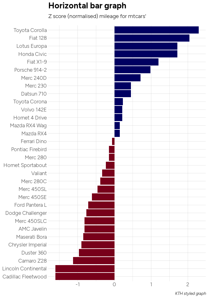
Diverging colors:
cars <-
  mtcars %>%
  mutate(brand = rownames(mtcars)) %>%
  mutate(mpg_z_score = (mpg - mean(mpg, na.rm = TRUE)) / sd(mpg)) %>%
  mutate(mpg_type = ifelse(mpg_z_score < 0, "below", "above")) %>%
  mutate(CarBrand = factor(mpg_type, levels = unique(mpg_type)))

pdiv <- palette_kth_neo(n = 7, type = "div")[c(1, 7)]
names(pdiv) <- NULL

ggplot(cars, aes(x=reorder(brand, mpg_z_score), y=mpg_z_score, label=mpg_z_score)) +
  geom_bar(stat='identity', aes(fill=mpg_type)) +
  scale_fill_manual(name="Mileage (deviation)",
    labels = c("Above Average", "Below Average"),
    values = c("above" = pdiv[1], "below" = pdiv[2])) +
  labs(subtitle="Z score (normalised) mileage for mtcars'",
    title= "Horizontal bar graph", caption="KTH styled graph") +
  theme_kth_neo() +
  theme(
    axis.title.y=element_blank(),
    axis.title.x=element_blank(),
    legend.position="none"
  ) +
  coord_flip()
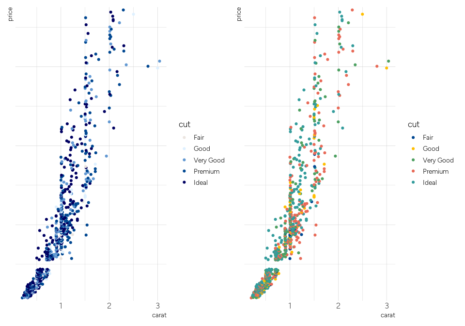
Sequential discrete colors versus qualitative discrete colors:
library(patchwork)

pdiv <- rev(tolower(palette_kth_neo(n = 5, type = "seq") %>% setNames(NULL)))
dsamp <- diamonds[1 + 1:1000 * 50, ]

gg <- ggplot(dsamp, aes(carat, price, color = cut)) + geom_point()

gg1 <- gg + scale_color_manual(values = pdiv) +
  theme_kth_neo() + scale_y_comma()

gg2 <- gg + scale_color_kth() +
  theme_kth_neo() + scale_y_comma()

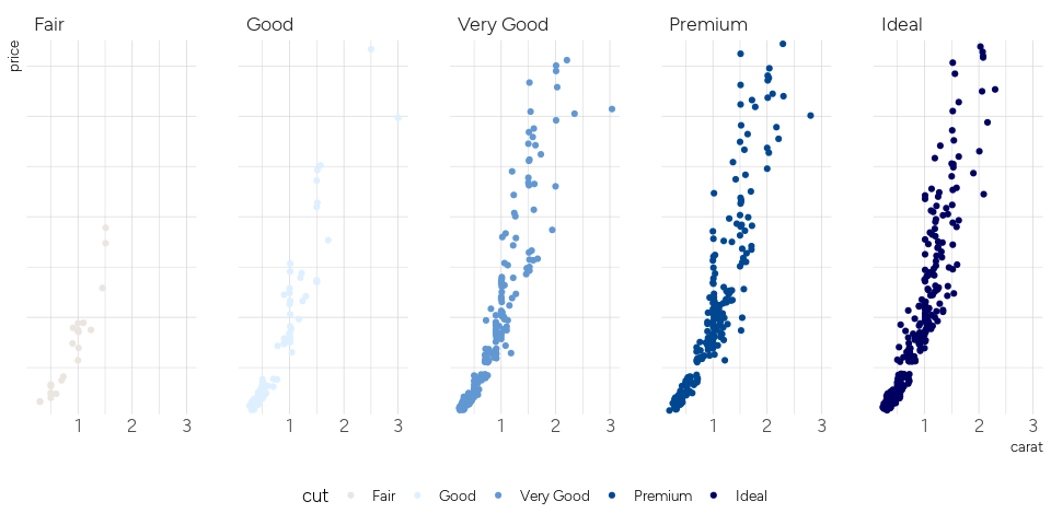
gg3 <- gg + facet_wrap(~cut, ncol = 5) + scale_color_manual(values = pdiv) +
  theme_kth_neo() + scale_y_comma() + theme(legend.position="bottom")

gg1 + gg2
In this case it might be better to use small multiples (like below) or another type of visual.
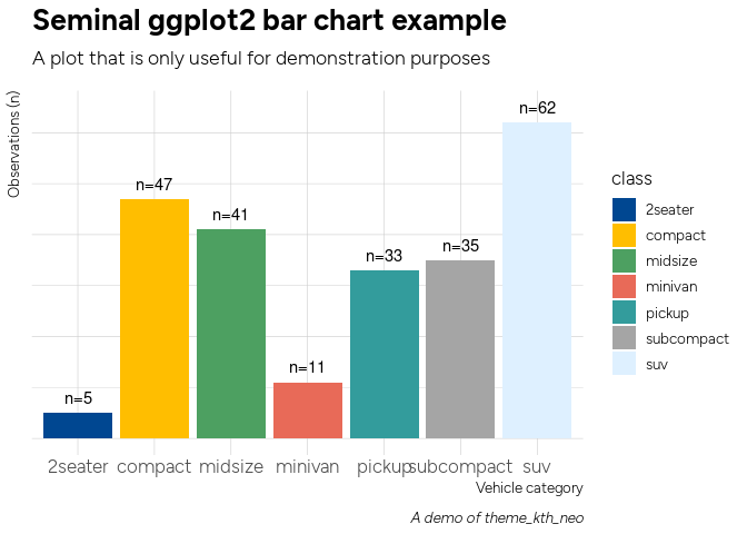
gg3Another example with a simple bar plot:
#update_geom_font_defaults(family=font_osc)
#import_open_sans_condensed()
#extrafont::loadfonts()

# library(readr)
# ft <- read_csv(system.file("fontmap", "fonttable.csv", package="extrafontdb"))
# regular_osc <- ft %>% filter(FamilyName == "Open Sans Condensed") %>% head(1)
# regular_osc$FullName <- "Open Sans Condensed"
# regular_osc$Bold <- FALSE
# ft_new <- bind_rows(ft, regular_osc)
# write_csv(ft_new, path = system.file("fontmap", "fonttable.csv", package="extrafontdb"))

library(dplyr)
library(ggplot2)

count(mpg, class) %>%
ggplot(aes(class, n)) +
geom_col(aes(fill = class)) +
geom_text(aes(label=paste0("n=", n)), nudge_y=3) +
labs(x="Vehicle category", y="Observations (n)",
     title="Seminal ggplot2 bar chart example",
     subtitle="A plot that is only useful for demonstration purposes",
     caption="A demo of theme_kth_neo") +
theme_kth_neo() +
scale_fill_kth() +
theme(axis.text.y=element_blank())
Examples of customized ggplots used in the R package bibliomatrix:
# library(dplyr)
# library(patchwork)
# suppressPackageStartupMessages(library(bibliomatrix))
# abm_public_kth <- bibliomatrix::abm_public_data()
#
# # Fetching som data from bibliomatrix::abm_public_kth
# cf <- abm_public_kth$units$KTH[[3]] %>% filter(interval == "Total") %>% pull(cf)
#
# # this is a ggplot2-based bullet graph
# p1 <-
#   abm_bullet(label = "Field normalized citations (Cf)",
#   value = cf, reference = 1.0, roundto = 2) +
#     theme_kth() +
#     # override some theme settings
#     theme(
#       plot.title=element_text(size = 12),
#       axis.text.x=element_text(size = 8),
#       axis.title.x=element_blank(),
#       axis.title.y=element_blank(),
#       axis.line.y=element_blank(),
#       axis.line.x=element_blank(),
#       axis.text.y=element_blank(),
#       axis.ticks.x=element_blank(),
#       panel.grid.major=element_blank(),
#       panel.grid.minor=element_blank()
#     )
# nonuniv_share <-
# abm_public_kth$units$KTH[[5]] %>% filter(interval == "Total") %>% pull(nonuniv_share)
#
# nonuniv_lbl <-
# sprintf("Swedish non-university: %d%%", round(100 * nonuniv_share))
#
# # this is a ggplot2-based waffle chart
# p2 <- abm_waffle_pct(nonuniv_share, label = nonuniv_lbl) +
# theme_kth() +
# # override some theme settings
# theme(
# axis.text.y=element_blank(),
# axis.text.x=element_blank(),
# legend.position="none"
# )
#
# p1 + p2
#
#
# # this is a pie - saved for last, the dessert
#
# df <- data.frame(
# group = c("Male", "Female", "Child"),
# value = c(25, 25, 50)
# )
#
# pie <-
# ggplot(df, aes(x = "", y = value, fill = group)) +
# geom_bar(width = 1, stat = "identity") +
# coord_polar("y", start = 0) +
# scale_fill_manual(values = unname(ktheme::palette_kth()), guide = FALSE) +
# theme_kth_osc(base_family = "Open Sans Condensed Light") + theme(
# axis.title.x = element_blank(),
# axis.title.y = element_blank(),
# panel.border = element_blank(),
# panel.grid = element_blank(),
# axis.ticks = element_blank()
# ) +
# geom_text(aes(y = value / 3 + c(0, cumsum(value)[-length(value)]),
# label = sprintf("%s\n(%s)", group, scales::percent(value / 100))), size = 5)
#
# pie


