JosueMA / mcp

Bayesian inference of Multiple Change Points

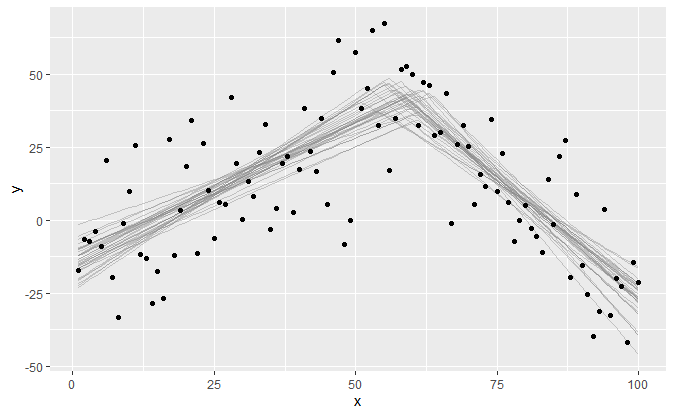
Bayesian inference of multiple change points and the parameters of the (linear) segments in between. Under the hood, mcp takes an abstract representation of linear segments and turns it into JAGS code. The rest of the package ensures seamless compatibility with your favourite Bayesian packages, including tidybayes, bayesplot, and loo.

You can see the roadmap for the immediate future under issues. Expect breaking changes in the API until version 1.0. Also be aware that it has not been thoroughly tested. I would be very excited about any feedback, positive or negative or constructive. Please raise issues or contact me elsewhere, e.g., @jonaslindeloev on Twitter or firstname at lindeloev.dk.

Install

1. Install the latest version of JAGS. Linux users can fetch binaries here.

2. Install mcp by running this in R: devtools::install_github("lindeloev/mcp"). If you don't have devtools, install it first using install.packages("devtools").

Quick example

Find the single change point between two joined slopes:

# Define segments
segments = list(
    y ~ 1 + x,  # intercept + slope
    1 ~ 0 + x  # joined slope
)

# Start sampling
fit = mcp(segments, my_data)

# Plot fit
plot(fit)

Extended guide

Let us specify a fairly complicated model with four segments, i.e., three change points:

# Define the segments that are separated by change points
segments = list(
  score ~ 1 + year,  # intercept + slope
  1 ~ 0 + year,  # joined slope
  1 ~ 0,  # joined plateau
  1 ~ rel(1)  # disjoined plateau with relative intercept parameterization
)

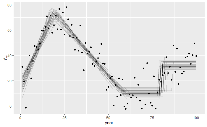
This is what we will end up with. We simulate some raw data from this model (the points) and infer the parameter of the linear segments as well as the change points (lines are draws from the posterior distribution).

This model has the following parameters:

• cp_1, cp_2, and cp_3: change points on the x-axis (here year). One between each adjacent segment.
• int_1 and int_4: intercept changes on y (here score). Only specified in the first and the last segment.
• year_1, year_2: slopes in segments 1 and 2. Takes name after the x-axis predictor.
• sigma: standard deviation of residuals.

Simulate data using fit$func_y()

It will usually be a good idea to run mcp without sampling first, in which case it returns a full mcpfit object without samples. This contains a list of priors (mcp$prior), JAGS code (fit$jags_code), and an R function of the model (mcp$func_y()).

We can use the latter to simulate data. This is always a great way to get acquainted with new models and functions, and ensure that they can recover the parameters.

# Get an mcpfit object without samples
fit_empty = fit(segments, sample=FALSE)

# Now use fit_empty$func_y() to generate data from this model.
# Set some parameter values to your liking:
data = data.frame(
  year = 1:100,  # Evaluate func_y for each of these
  score = fit_empty$func_y(
    year = 1:100,  # x
    sigma = 12,  # standard deviation
    cp_1 = 20, cp_2 = 55, cp_3 = 80,  # change points 
    int_1 = 20, int_4 = 20,  # intercepts
    year_1 = 3, year_2 = -5  # slopes
  )
)

Set priors

Quite uninformative priors are set using data by default. You can see them in fit$prior. We can override some or all of these by providing JAGS code.

prior = list(
  int_1 = "dunif(10, 30)",  # intercept of segment 1
  cp_2 = "dunif(cp_1, 40)",  # change point between segment 1 and 2 is before 40.
  year_2 = "dnorm(0, 5)"  # slope of segment 1.
)

mct has a few tricks up the sleeve for setting priors.

• Order restriction is automatically applied to cp_* parameters using truncation (e.g., T(cp_1, )) so that they are in the correct order on the x-axis UNLESS you do it yourself. The one exception is for dunif distributions where you have to do it as above.

• In addition to the model parameters, MINX (minimum x-value), MAXX (maximum x-value), SDX (etc...), MINY, MAXY, and SDY are also available when you set priors. They are used to set uninformative default priors.

• Use SD when you specify priors for dt, dlogis, etc. JAGS uses precision but mct converts to precision under the hood via the sd_to_prec() function.

Fit the model

This is the easiest step!

fit = mcp(segments, data, prior)
fit 

# A tibble: 8 x 4
  name    mean .lower .upper
  <chr>  <dbl>  <dbl>  <dbl>
1 cp_1   18.5   15.9   20.7 
2 cp_2   56.7   42.2   67.7 
3 cp_3   68.6   46.0   96.0 
4 int_1  11.3    1.17  21.7 
5 int_4  16.4   11.0   22.2 
6 sigma  11.7   10.0   13.4 
7 year_1  3.72   2.76   4.74
8 year_2 -5.54  -6.65  -4.45

(This summary is very preliminary and will be updated)

Plots

Let us inspect it visually:

plot(fit)

By default this draws lines given 25 posterior samples, but change it using plot(fit, draws=50). Of particular interest is how similar the lines are (good precision) and how well they fit to the data. plot.mcpfit returns a ggplot2 object, so you can easily add, e.g., a title: plot(fit, "combo") + ggtitle("Posteriors and convergence").

We may also want to inspect the posterior distributions directly:

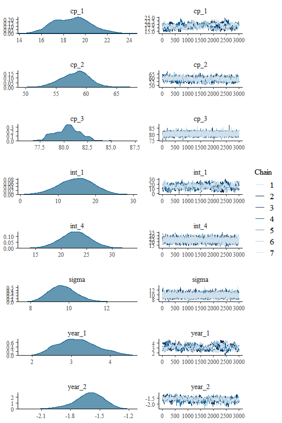
plot(fit, "combo")

This is a classical Bayesian plot to better see parameter estimates and to check convergence between chains. Compare the inferred values to the one we used to generate the data. Change point models do a remarkably good job of recovering the change points on other parameters, including sigma.

Notice that int_4 was modeled as relative (rel(1)) so it is the difference from the change point. It would have had a different value if it was modeled as absolute (1).

If you need to increase the warmup or number of post-warmup iterations, mcp(...) are channeled directly to jags.fit, so you can do mcp(segments, data, n.adapt = 3000, n.update = 3000, n.iter = 5000).

Model comparison

Now it's time for some model comparison. We will compare to an intercept-only model with default priors. This one has no change points because there is only one segment, i.e., it is a classical linear regression model. Because the x-axis cannot be read out from the segments when there are no slopes, we need to give it explicitly:

segments2 = list(score ~ 1)
fit2 = mcp(segments2, data, param_x = "year")

We can use the cross-validation from the loo package to compare the predictive performance of various models. We compute loo for each model and then compare them. the mcpfit objects have placeholders for loo and waic fits. You need not use them, but it's nice to keep things together:

fit$loo = loo(fit)
fit2$loo = loo(fit2)
loo_compare(fit$loo, fit2$loo)

Result:

       elpd_diff se_diff
model1   0.0       0.0  
model2 -47.0      10.0 

Aha, the first model in loo_compare (fit) was preferred (higher Estimated Log-Predictive Density). The important thing here is the elpd_diff/se_diff ratio. This is almost like a z-score, i.e., a ratio of 1.96 corresponds to 95% probability that fit has superior predictive accuracy. BUT, the loo developers have adviced that it is probably too optimistic in practice, so that one should only begin taking it seriously if this ratio exceeds 5 [Citation needed].

... and more

Lastly, don't be constrained by these simple mcp functions. You can work with the MCMC samples just as you would with brms, stan_glm, jags, or other samplers using the always excellent tidybayes:

library(tidybayes)

# Extract all parameters:
tidy_draws(fit$samples) %>%
  # tidybayes stuff here

# Extract some parameters:
fit$pars$model  # check out which parameters are inferred.
spread_draws(fit$samples, cp_1, cp_2, int_1, year_1) %>%
 # tidybayes stuff here