Jonas1312 / dilation-rate-as-fibonacci-sequence

Dilation Rate Gridding Problem and How to Solve It With the Fibonacci Sequence.

Dilation Rate Gridding Problem and How to Solve It With the Fibonacci Sequence

Introduction

In convolutional neural networks, it is assumed that the receptive field must cover a sufficiently large area of the input image, so that the last layers of the network can have a global overview of the elements present in it.

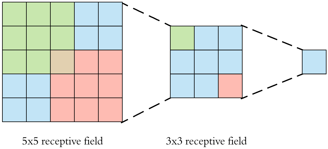
On the figure below, we see how stacking two 3x3 convolutions will result in a 5x5 receptive field with 18 parameters (3x3 + 3x3 = 18):

There's usually 3 common ways to increase the receptive field:

1. more layers
2. pooling with strides
3. dilated convolutions.

The most used technique is to add a pooling layer. It's indeed very effective at increasing the receptive field without any added computational cost.

However, pooling can cause several issues such as breaking the Shannon-Nyquist sampling theorem. It also, by definition, provokes a loss of data which can be undesirable when we need to preserve the original image resolution.

The other technique uses dilated convolutions:

Dilated convolutions preserve the number of parameters and the resolution, while effectively increasing the receptive field.

However, they also come with an interesting issue: the gridding problem.

Problematic

Let's do some visualizations using Python and PyTorch to see how the gridding problem appears.

Some imports:

%matplotlib inline
import io

import imageio
import matplotlib.pyplot as plt
import numpy as np
import PIL
import torch

Settings for plotting:

plt.rcParams["figure.facecolor"] = (1.0, 1.0, 1.0, 1)
plt.rcParams["figure.figsize"] = [3, 3]
plt.rcParams["figure.dpi"] = 150
plt.rcParams["legend.fontsize"] = "large"
plt.rcParams["axes.titlesize"] = "large"
plt.rcParams["axes.labelsize"] = "large"
plt.rcParams["xtick.labelsize"] = "small"
plt.rcParams["ytick.labelsize"] = "small"

Below, we create a function that generates a neural network with $N$ convolution layers with respective dilation rates defined as a parameter:

def generate_network(dilation_rates: list):
    layers = []
    for dilation in dilation_rates:
        conv = torch.nn.Conv2d(
            in_channels=1,
            out_channels=1,
            kernel_size=3,
            stride=1,
            padding="same",
            dilation=dilation,
            bias=False,
            padding_mode="zeros",
        )
        conv.weight.data.fill_(1)
        layers.append(conv)
    network = torch.nn.Sequential(*layers)
    return network

We also need another function that:

1. initializes the network
2. creates the input image
3. computes the output
4. returns the gradient of the output center pixel with respect to the input image.

def inference_and_return_grad(pixels: int, dilation_rates: list):
    net = generate_network(dilation_rates)

    input_image = torch.zeros((1, 1, pixels, pixels))
    input_image.requires_grad_(True)

    output = net(input_image)

    # we return the gradient of the output pixel center
    # with respect to the input image
    center_pixel = output[0, 0, pixels // 2, pixels // 2]
    center_pixel.backward()
    return input_image.grad

We define the input as a 21x21 pixels image:

pixels = 21

We create a function to help with plotting the gradient.

For all visualizations below:

• white pixels have no impact on the output center pixel
• blue pixels have an impact on the output center pixel, the darker the blue, the greater the impact.

def plot_grad(grad, title, show=True):
    grad = grad[0, 0]
    ax = plt.imshow(grad, cmap="Blues", interpolation="none")
    plt.title("Dilation rates: " + title)
    if show:
        plt.show()
    else:
        return ax

We start with plotting the gradient of the output center pixel w.r.t. the input pixels for a 3-layers convolutional network without dilation ( $dilation=1$ ):

plot_grad(
    inference_and_return_grad(pixels, dilation_rates=(1, 1, 1)), title="(1, 1, 1)"
);

Looks good to me, it's a classic 3-layers CNN with 3x3 kernels...

Now, let's try to reproduce the gridding problem with a 4-layers CNN and a dilation rate of 2:

plot_grad(
    inference_and_return_grad(pixels, dilation_rates=(2, 2, 2, 2)), title="(2, 2, 2, 2)"
);

We can see that the output center pixel has a big receptive field encompassing the whole image, which is the purpose of dilated convolutions.

However, we also clearly notice a uniform grid of pixels not contributing to the output center pixel, which is the unwanted gridding problem.

In some neural network architectures, we sometimes see successive dilation rates growing exponentially:

plot_grad(
    inference_and_return_grad(pixels, dilation_rates=(1, 2, 4)), title="(1, 2, 4)"
);

This shouldn't be used since we can see that some pixels contribute more to the output center pixel than the input center pixel itself.

Solution

The key to solve the gridding problem is to use the Fibonacci sequence.

We can see that it effectivily solves the gridding issue:

plot_grad(
    inference_and_return_grad(pixels, dilation_rates=(1, 1, 2, 3, 5)),
    title="(1, 1, 2, 3, 5)",
);

def fibonacci_sequence(seq_len: int):
    fib_seq = [1, 1]
    for _ in range(seq_len - 2):
        fib_seq.append(fib_seq[-1] + fib_seq[-2])
    return fib_seq

We can visualize the impact on the gradient of adding several conv layers with dilation rates following the Fibonacci sequence:

%%capture
writer = imageio.get_writer("anim.gif", mode="I", duration=1)

nb_layers_end = 6
fib_seq = fibonacci_sequence(nb_layers_end)

for nb_layers in range(1, nb_layers_end + 1):
    ax = plot_grad(
        inference_and_return_grad(pixels, dilation_rates=fib_seq[:nb_layers]),
        show=False,
        title=str(fib_seq[:nb_layers]),
    )
    buf = io.BytesIO()
    ax.figure.savefig(buf, dpi=150)
    buf.seek(0)
    pil_img = PIL.Image.open(buf)
    writer.append_data(np.array(pil_img))