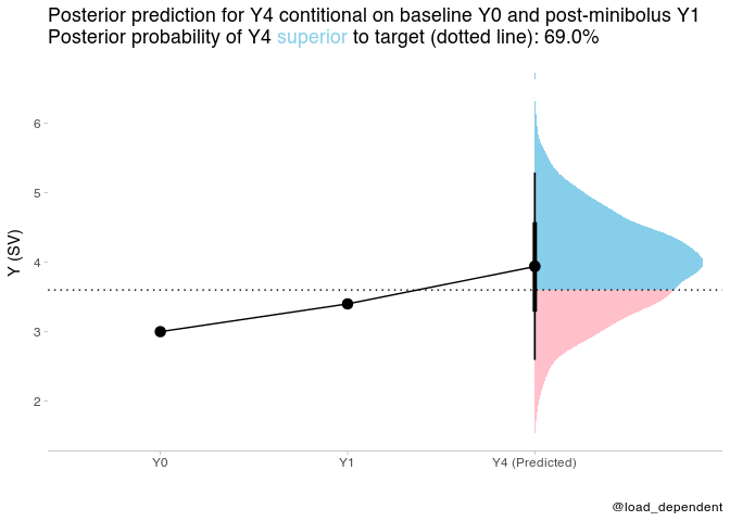
Simulation of fluid responsiveness prediction trial, by mini-fluid boluses, using predictions from a bayesian linear model.
Shiny app for interactive simulation
Simulate data, based on this datamethods.org discussion
set.seed(1349)

n <- 1000
# true values
Y0 <- rnorm(n, 5, 1)

a <- rnorm(n, 0, 1) # change
Y1 <- Y0 + a/2
Y4 <- Y1 + a

# add independent random noise
Y0 <- Y0 + rnorm(n, 0, 0.2)
Y1 <- Y1 + rnorm(n, 0, 0.2)
Y4 <- Y4 + rnorm(n, 0, 0.2)
df <- tibble(Y0,Y1,Y4)
Fit models, using flat priors (for simplicity)
model1 <- brm(Y4 ~ 0 + Y0 + Y1,
          data = df,
          file = here("fluid_response","model1.Rds"),
          file_refit= "on_change"
          )
model1
## Family: gaussian
## Links: mu = identity; sigma = identity
## Formula: Y4 ~ 0 + Y0 + Y1
## Data: df (Number of observations: 1000)
## Samples: 4 chains, each with iter = 2000; warmup = 1000; thin = 1;
## total post-warmup samples = 4000
##
## Population-Level Effects:
## Estimate Est.Error l-95% CI u-95% CI Rhat Bulk_ESS Tail_ESS
## Y0 -1.37 0.04 -1.44 -1.30 1.00 1271 1585
## Y1 2.37 0.04 2.30 2.44 1.00 1288 1546
##
## Family Specific Parameters:
## Estimate Est.Error l-95% CI u-95% CI Rhat Bulk_ESS Tail_ESS
## sigma 0.68 0.02 0.65 0.71 1.01 1758 1667
##
## Samples were drawn using sampling(NUTS). For each parameter, Bulk_ESS
## and Tail_ESS are effective sample size measures, and Rhat is the potential
## scale reduction factor on split chains (at convergence, Rhat = 1).
New values for Y0 and Y1 to predict Y4 from, and minimum SV to target
Y0_new <- 3.0
Y1_new <- 3.4
Y4_target <- 3.6 #minimum co target
Generate posterior predictions based on Y0 and Y1
prediction <- tibble(Y0=Y0_new,Y1=Y1_new) %>%
  add_predicted_draws(model1)

head(prediction)
## # A tibble: 6 × 7
## # Groups: Y0, Y1, .row [1]
## Y0 Y1 .row .chain .iteration .draw .prediction
## <dbl> <dbl> <int> <int> <int> <int> <dbl>
## 1 3 3.4 1 NA NA 1 4.53
## 2 3 3.4 1 NA NA 2 4.81
## 3 3 3.4 1 NA NA 3 3.80
## 4 3 3.4 1 NA NA 4 4.03
## 5 3 3.4 1 NA NA 5 4.16
## 6 3 3.4 1 NA NA 6 2.94
Calculate posterior probability of Y4 superior to target
post_pred_prob <- prediction %>%
  summarise(prob=mean(.prediction>Y4_target)) %>%
  pull(prob)
## `summarise()` has grouped output by 'Y0', 'Y1'. You can override using the `.groups` argument.
Data for points and lines
plot_data = tibble(time=ordered(c("Y0","Y1","Y4 (Predicted)")),y=c(Y0_new,Y1_new,mean(prediction$.prediction)),group="group")plot_data %>%
ggplot(aes(x = time, y = y,group="group")) +
stat_halfeye(aes(y = .prediction, x = "Y4 (Predicted)", fill = after_stat(ifelse(y > Y4_target, "over", "under"))), data = prediction) +
geom_point(size=3)+
geom_path()+
geom_hline(yintercept = Y4_target,linetype="dotted")+
scale_fill_manual(values = c("over" = "#87ceeb", "under" = "#FFC0CB")) +
scale_y_continuous(name = "Y (SV)")+
scale_x_discrete(name="")+
theme_tidybayes() +
labs(title = paste0(
"Posterior prediction for Y4 contitional on baseline Y0 and post-minibolus Y1 <br>",
"Posterior probability of Y4 <span style='color:#87ceeb;'>superior</span> to target (dotted line): ", scales::percent(post_pred_prob, accuracy = .1)
),caption = "@load_dependent") +
theme(
legend.position = "none", axis.line.y = NULL,
plot.title = element_markdown(lineheight = 1.1),
legend.text = element_markdown(size = 11)
)We can also fit the model using change from Y0 to Y1 I(Y1 - Y0) and
the mean I((Y1 + Y0) / 2) of the two values.
model2 <- brm(Y4 ~ 0 + I(Y1 - Y0) + I((Y1 + Y0) / 2),
          data = df,
          file = here("fluid_response","model2.Rds"),
          file_refit= "on_change"
          )
model2
## Family: gaussian
## Links: mu = identity; sigma = identity
## Formula: Y4 ~ 0 + I(Y1 - Y0) + I((Y1 + Y0)/2)
## Data: df (Number of observations: 1000)
## Samples: 4 chains, each with iter = 2000; warmup = 1000; thin = 1;
## total post-warmup samples = 4000
##
## Population-Level Effects:
## Estimate Est.Error l-95% CI u-95% CI Rhat Bulk_ESS Tail_ESS
## IY1MY0 1.87 0.04 1.79 1.95 1.00 3308 2886
## IY1PY0D2 1.00 0.00 0.99 1.01 1.00 4722 3222
##
## Family Specific Parameters:
## Estimate Est.Error l-95% CI u-95% CI Rhat Bulk_ESS Tail_ESS
## sigma 0.68 0.02 0.65 0.71 1.00 2948 2814
##
## Samples were drawn using sampling(NUTS). For each parameter, Bulk_ESS
## and Tail_ESS are effective sample size measures, and Rhat is the potential
## scale reduction factor on split chains (at convergence, Rhat = 1).
The estimate for I((Y1 + Y0) / 2) is 1, indicating that the expected
difference between the Y4 and the mean of Y1 and Y0 only depend on the
difference between Y0 and Y1. I.e. with this simulated data, we only
need to consider the change from Y0 to Y1 to predict the change from
mean(Y0, Y1) to Y4 (which is similar to the current use of the MFC
approach).
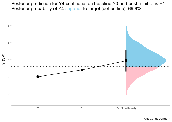
I believe the models are equivalent though, so it should be possible to draw the same insight from the more attractive model 1.
The following is just the same predictions as above, but for model 2. They are equivalent.
Generate posterior predictions based on Y0 and Y1
prediction2 <- tibble(Y0=Y0_new,Y1=Y1_new) %>%
  add_predicted_draws(model2)

head(prediction2)
## # A tibble: 6 × 7
## # Groups: Y0, Y1, .row [1]
## Y0 Y1 .row .chain .iteration .draw .prediction
## <dbl> <dbl> <int> <int> <int> <int> <dbl>
## 1 3 3.4 1 NA NA 1 4.83
## 2 3 3.4 1 NA NA 2 5.85
## 3 3 3.4 1 NA NA 3 3.94
## 4 3 3.4 1 NA NA 4 2.80
## 5 3 3.4 1 NA NA 5 3.64
## 6 3 3.4 1 NA NA 6 3.92
Calculate posterior probability of Y4 superior to target
post_pred_prob2 <- prediction2 %>%
  summarise(prob=mean(.prediction>Y4_target)) %>%
  pull(prob)
## `summarise()` has grouped output by 'Y0', 'Y1'. You can override using the `.groups` argument.
Data for points and lines
plot_data2 = tibble(time=ordered(c("Y0","Y1","Y4 (Predicted)")),y=c(Y0_new,Y1_new,mean(prediction2$.prediction)),group="group")plot_data2 %>%
ggplot(aes(x = time, y = y,group="group")) +
stat_halfeye(aes(y = .prediction, x = "Y4 (Predicted)", fill = after_stat(ifelse(y > Y4_target, "over", "under"))), data = prediction2) +
geom_point(size=3)+
geom_path()+
geom_hline(yintercept = Y4_target,linetype="dotted")+
scale_fill_manual(values = c("over" = "#87ceeb", "under" = "#FFC0CB")) +
scale_y_continuous(name = "Y (SV)")+
scale_x_discrete(name="")+
theme_tidybayes() +
labs(title = paste0(
"Posterior prediction for Y4 contitional on baseline Y0 and post-minibolus Y1 <br>",
"Posterior probability of Y4 <span style='color:#87ceeb;'>superior</span> to target (dotted line): ", scales::percent(post_pred_prob2, accuracy = .1)
),caption = "@load_dependent") +
theme(
legend.position = "none", axis.line.y = NULL,
plot.title = element_markdown(lineheight = 1.1),
legend.text = element_markdown(size = 11)
)
