There was a lot to write about this two stage project/investigation. You can use the TOC (generated with gh-md-toc) to navigate.
Super resolution imaging has a wide application from satellite imaging to photography. However, how I got exposed to it is due to wanting to use an image as my mobile phone's wallpaper when it had low resolution. The idea of some kind of fully-convolutional encoder-decoder network came to me and of course, a number of papers have already been published around this topic. With some experience in implementing CycleGAN and DCGAN (GANs repo), I read some relevant resources and started diving into the rabbit hole of image super resolution.
Overall, I built and trained a Photo-Realistic Single Image Super-Resolution Generative Adversarial Network with TensorFlow + Keras and investigated the importance of the training dataset using Fréchet Inception Distance as the evaluation metric. Being able to extract enough information from heavily downsized 44x44 photos with complex geometry (human face) to realistic 176x176 portraits, the final model has surpassed human-level performance.
   LR (low-res)            Bicubic           SR (Model A)          SR (Model B)        HR (high-res)
         |                     \___________________|___________________/                      |
         |                                         |                                          |
    Input Image              Ways of Increasing Resolution (SR = super-res)            Ground Truth
Stage 1: the goal is to map 44x44 colored images to size 176x176 (upsampling factor of 4) while keeping the perceptual details and textures. The main source of knowledge came from the original SRGAN paper and an analysis on the importance of dataset. Despite not having compatible hardware for the computational demanding models, I achieved great results by using smaller images, tweaking the model configuration, and lowering the batch size. One unfortunate occurance is that I and my model found out the hard way that it was impossible for 44x44 images to capture the complexity of human face. However, the model persisted and still pumped out visually convincing results.
Stage 2: this is an investigation to answer my own question of "whether the range of dataset content matter". I trained two identical models (Model A and Model B) separately on the COCO dataset (high content variance) and the CelebA dataset (specific "face" category of content), then used visual results and Fréchet Inception Distance to both qualitatively and quantitatively demonstrate the results of my investigation.
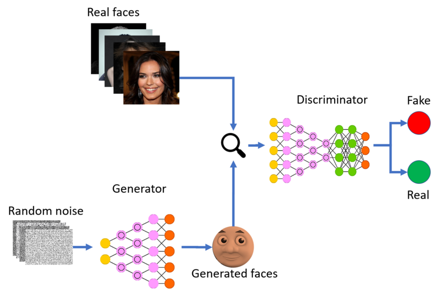
Invented by Ian GoodFellow in 2014, GAN showed amazing image generative abilities by making completely new images from road scenes to faces. However, generating images out of random noise is only a fraction of its capability. From switching images between domains (CycleGAN) to music generation (MidiNet), the breadth of tasks GAN could take on is still being discovered.
Single image super resolution (SISR) can be defined as upscaling images while keeping the drop in quality to minimum, or restoring high resolution images from details obtained from low resolution images. Traditionally, this was done with mostly bicubic interpolation (video: cubic spline). However, interpolation has the tendency of making images blurry and foggy. Utilizing deep learning techniques, SRGAN learns a mapping from the low-resolution patch through a series of convolutional, fully-connected, and transposed/upsampling convolutional layers into the high-resolution patch while keeping texture/perceptual details. It greatly surpassed the performance of any traditional methods. It has applications in the fields of surveillance, forensics, medical imaging, satellite imaging, and photography. The architecture of SRGAN could also be used for image colorization and edge to photo mapping.
Below is my attempt to concisely explain everything about SRGAN with some images/diagrams from the original paper and various blogs. The model borrowed a lot of up to date techniques from various published papers, such as residual networks and PReLU (parameterized ReLU).
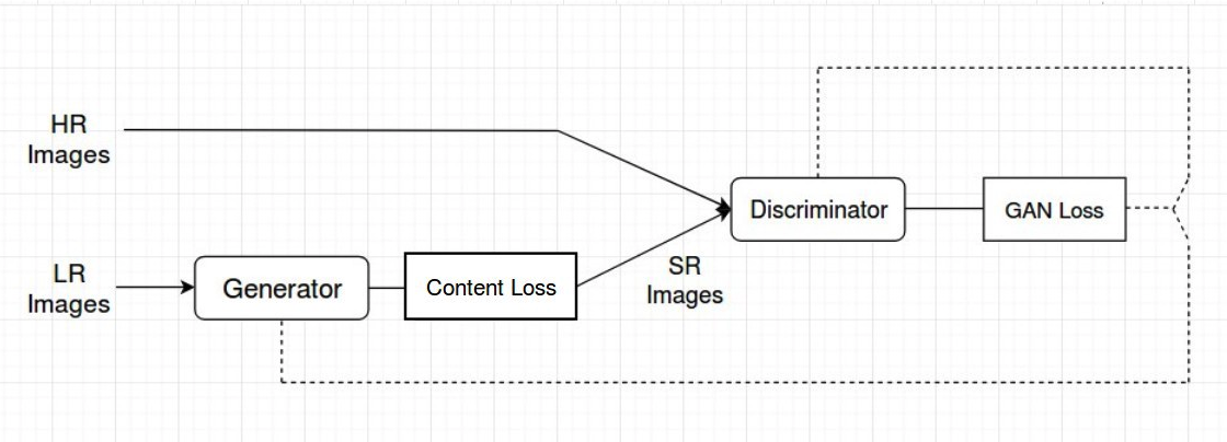
GAN is an unsupervised ML algorithm that employs supervised learning for training the discriminator (most of the time BCE). The high level architecture of SRGAN closely resembles the vanilla GAN architecture and is also about reaching the Nash Equilibrium in a zero-sum game between the generator and the discriminator. However, this is certainly not the only form GAN can take on, check out CycleGAN where 2 generators and 2 discrimintors were needed. Below are the high level procedures.
- High resolution (HR) ground truth images get selected from the training set
- Low resolution (LR) images are created with bicubic downsampling
- The generator upsamples the LR images to Super Resolution (SR) images to fool the discriminator
- The discriminator distinguishes the HR images (ground truth) and the SR images (output)
- Discriminator and generator trained with backpropagation
The generator takes a LR image, process it with a Conv and a PReLU (trainable LReLU) layer, puts it through 16 residual blocks borrowed from SRResNet, upsamples by factor of 2 twice, and puts it through one last conv layer to produce the SR image. Unlike normal convolutional layers, going crazy with the number of residual blocks is not prone to overfitting the dataset because of identity mapping.
The discriminator is similar to a normal image classifier, except its task is now more daunting due to having to perform binary-classification two images with near identical content (if the generator is trained well enough). It puts HR and SR images first through a Conv and a LReLU layer, process the image through 7 Conv-BN-LReLU blocks, flatten the image, then uses two dense layers with a LReLU in the middle and a sigmoid function at the end for classification.
At first I thought despite identity mapping, 16 residual blocks and 7 discriminator blocks was an overkill to produce a 176x176 image. However, it does make sense because the generator needs to learn the features of an image well enough to the point of producing a more detailed version of it. On the other hand, the discriminator has to classify two images with increasingly identical content converging toward being the absolute same.
On top of all these, quoting Ian GoodFellow (podcast):
The way of building a generative model for GANs is we have a two-player game in the game theoretic sense and as the players of this game compete, one of them becomes able to generate realistic data.
Adversarial networks have to be constantly struggling against each other in this zero-sum game of GAN. The process of converging to the Nash Equilibrium can be extremely slow, that is one more reason for the large number of trainable parameters.
The equation above describes the goal of SRGAN - to find the generator weights/parameters that minimize the perceptual loss function averaged over a number of images. Inside the summation on the right side of the equation, the perceptual loss function takes two arguments - a generated SR image by putting an LR image into the generator function, and the ground truth HR image.
One of the major advantage DNN approach has over other numerical techniques for single image super resolution is using the perceptual loss function for backpropagation. It adds the content loss and 0.1% of the adversarial loss together then minimize them. Let's break it down.
Note:
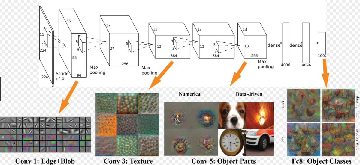
I do not fully agree with the feature extraction image on the right. Especially in much larger networks like SRGAN, discretizing what the neurons in each layer "look for" is impossible. Each layer of forward propagation should be seen as the network continuously understanding the image better and better, like how a brain learns by climbing a continuous slope instead of stepping on discrete stairs. However, the image does a good enough job visualizing why feature extraction is good for perceptual similarity.
Content loss refers to the loss of perceptual similarity between the SR and HR images. For many years people used MSE by default instead of this. However, minimizing MSE often produces blurry images as it is only based on pixel-to-pixel similarity, to computer the images might be similar, but human eyes extracts features from images instead of making pixel-wise calculations. Therefore, the original paper used the VGG19 network for feature extraction, then took the MSE of the extracted features instead.
Adversarial loss uses the classification results to calculate the loss of the generator. The formula provided by the paper is an augmented version of BCE loss for better gradient behavior. Instead, I experimented with the loss functions and chose to stick with BCE loss but tweaked the label value of SR images from 0 to a normal distribution around 0.1 to assist the discriminator's learning speed.
This section contains an overview of what I did, the problems I faced, and my solutions for overcoming them or at least mitigate them. I'll be referencing the background section quite a bit.
Preprocessing images from the COCO and CelebA datasets takes identical steps. I randomly selected images from each dataset, cropped the center out of raw images to serve as the high resolution data (ground truth), downsized them with Pillow's built in bicubic downsampling method to serve as the low resolution data (input), and normalized them before feeding them into the model. The code for these are in the beginning of the notebooks and in utils.py.
Being one of the newer applications of GAN when GAN is one of the newer neural architecture in the first place, the amount of resource on SRGAN was limited. Thankfully, the original paper was very informative and it did not contain any steep learning curves. For the model architecture, I mainly constructed the model from the original paper and experimented with the number of residual blocks and the loss functions (I ended up using BCE and tweaking the label value).
Refer to the background section for some detailed explanation of the architecture components and how they come together. For details on the parameters I used, I made a pretty neat list of them in parameters.txt. I also am quite fond of Keras' format for model summary especially compared to PyTorch's, I put the summaries in model_summary.txt to keep the notebooks short.
Hardware Performance
Even the creator of GAN, Ian Goodfellow himself would have thought of it as an infeasible idea due to simultaneously training two networks if he was not drunk (podcast, around 27 mins). Unfortunately, my experience showed that SRGAN is even worse because of its heavy and complex model configuration.
The actual training process failed multiple times due to the lack of computing power, GPU storage, and disconnection. These issues were resolved by:
Decreasing batch size, decreasing image sizes, uploading files from my local device, write outputs and models directly to Drive every few epochs, and having a "continue training" file with saved models (see files section for more details).
This is one of the most problematic project and I ended up learning a lot more about using Cloud Computing in general and obtained great results. After decreasing the image size and the dataset size to 2500 images (2000 train + 500 test), the provided T4 GPU ran at 4+ min/epoch and the total training time was more than a week for each model (2500 epochs).
Loss Analysis
The functions for parsing CelebA_loss.txt and COCO_loss.txt from loss is in utils.py. I observed these files to ensure that neither the generator nor the discriminator is dominating the game (having loss too close to 0). Sorry about the font size. The green curve is adversarial loss * 0.001, the orange curve is content loss, and the blue curve is the perceptual loss (sum of the previous two).
Loss of Model A (COCO dataset)
     _________________________________________________________/           \__________________________
    /                                                 Expand epoch 1500 - 1750                       \
Loss of Model B (CelebA dataset)
     _________________________________________________________/           \__________________________
    /                                                 Expand epoch 1500 - 1750                       \
When the figures above were plotted with matplotlib, I was first disappointed as there seemed to be no decrease of content/generator loss beyond epoch 500 and it did not look like the generator and discriminator were struggling against each other like this one). However, when I zoomed into smaller segments of the graph, it became clear that the height of initial content loss made the continuously decreasing content loss and the struggles between content loss and adversarial loss too small to see.
The content loss steadily decreased throughout the 2500 epochs for both models trained on COCO and CelebA. Indicating that gradient descent is not overshooting and the model weights are moving toward the Nash equilibrium (content loss of ~0 and discriminator can only have 50% guessing chance). However, tuning hyperparameter was hard since each try forfeits days of training progress. This blog also explains why GAN is harder to train than most other neural architectures.
One more thing to notice is that the content loss of Model A was consistently approximately 2x of Model B. This can be explained by the high variety of COCO dataset content making it very hard for the model to optimize its losses.
Model A (Trained on COCO)
I trained the Model A on the COCO dataset and quickly noticed the issue of it performing badly with details mostly due to 44x44 images not capturing enough texture and perceptual details (fur, patterns, etc). Due to the fact that Human face is the most complex feature that can appear in a picture, Model A's performance on it is often absolutely atrocious. Since I already wanted to investigate whether how the range of dataset content affect a model's performance, I chose to train my second model completely on faces with the CelebA dataset to observe just how much I can push the generator to extract the complex features of human face packed inside a 44x44 image.
Image with more details:
LR (low-res) Bicubic SR (Model A) SR (Model B) HR (high-res)
Image with less details:
Model B (Trained on CelebA)
Model B was trained with only facial images and it already started producing realistic human faces by the 500th epoch, thanks to the low variance of training content. However, it struggled with the most detailed but a very important feature of human face - the eyes. Since the downsized images compressed eyes into just few black pixels, reconstructing the eyes of people was virtually impossible. Gradually, the generator learned what eyes look like and "drew" them onto the black pixels, just like how we would have dealt with this problem ourselves. Since the eyes are actually very important for recognizing faces, I continuously trained the model and observed a gradual improvement in the generator's ability in reconstructing/creating the eyes of people.
Example of when the drawn-on eyes are too narrow:
LR (low-res) Bicubic SR (Model A) SR (Model B) HR (high-res)
Additionally, teeth gaps and creases have also been causing similar troubles for the model. The struggles with these details can be traced back to not having more powerful hardware for processing bigger images and bicubic interpolation not being the optimal downsampling method for retaining perceptual information.
Performance Comparison between Bicubic Upsampling, Model A, and Model B
If I train model 1 with a variety of image contents and model 2 with only one category/type of images (dataset with narrower domain), say cats. Would model 2 perform better than model 1 on cat images or is SRGAN only about recognizing small textures and edges?
I asked this question on Quora and received no response :( and only later found out about this related paper, so I clarified my own question through experimentation. In the paper just mentioned, the researchers trained models on different categories of images (face, dining room, tower) to demonstrate that each model performs best on the category of images they were trained on with FID (Fréchet inception distance) as the evaluation metric. However, my question was not about training on different domains of image contents, but about training on a wide range of content vs. a narrow range of content (note that COCO dataset does contain many pictures of human faces, but a much bigger portion of it are not faces).
My investigation for this stage of the project can be simply put as:
If model A gets trained on images with a variety of contents (COCO) and model B gets trained with images in a specific domain of images (CelebA), how significant is the performance difference between A and B when evaluated on the images that model B was trained on?
Therefore, I trained two models with the same configuration separately on the COCO dataset and the CelebA dataset for the same number of epochs, then used FID to evaluate my models. FID is one of the most popular way to measure the performance of GAN and it compares the statistic of generated samples to real samples using the activations of an Inception-v3 network (details). The actual math is not too bad as long as you know what matrix trace is. Since it is a "distance" measurement (with multi-gaussian) between two images, lower FID indicates better performance and vice versa.
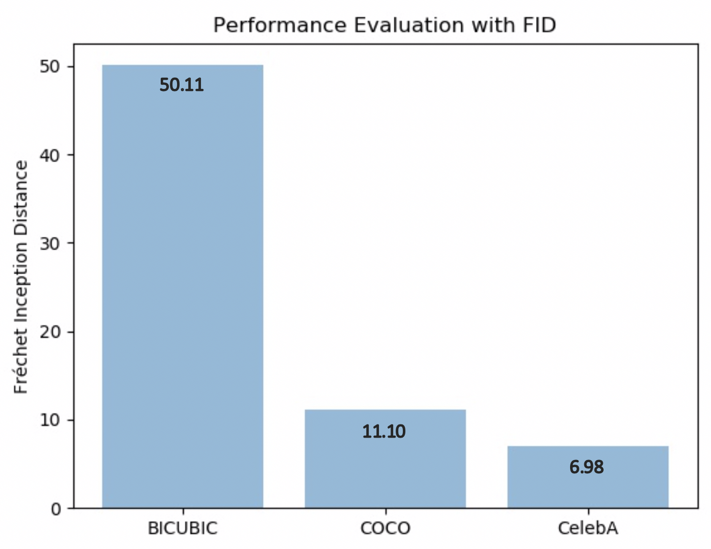
To measure the performance between bicubic upsampling (traditional method), model A, and model B on CelebA (the face images) test dataset (500 images), I first used the Pillow bicubic interpolation function and the two generators from both models to obtain three sets of super resolution images, then used the FID implementation from tsc2017 to measure their individual scores against the ground truth images. Then I produced the bar graph below.
The first thing to see here is that what a surprise, deep learning won against the traditional method. As could be seen among the results, bicubic upsampling greatly smoothens the image by fitting the image with cubic splines, causing its output to be very blurry. Using a less model-based approach, the SRGAN networks let neurons in each layer learn the images and thus provide more flexibility when mapping the low resolution images to super resolution.
The second thing to notice is that model B, purely trained on CelebA images, achieved 37% better on the CelebA images than model A, which is trained on a variety of images with human faces only constituting a portion of them. This shows that dataset indeed matters and upsampling images is not a task that could be simply done by recognizing edges and texture. However, judging by the difference between the FID score of bicubic and model A results, model A was still able to achieve almost 5 times better the performance than the traditional approach, which further demonstrates the power of neural networks qunatitatively.
Despite not having the best hardware, I am quite content with the quality of results my models gave me and about the fact that I was able to demonstrate everything I wanted with them. However, it is still important to keep in mind that the models would perform much better with more training epochs and images that are big enough to contain the information for reconstructing details like eyes or creases. Take a look at the original paper to see how impressive it could become.
Side note:
Despite that Model B was able to perform significantly better on the CelebA testing set than Model A was able to perform on anything specific. Model A was able to generalize into a much wider range of image contents and perform better on all of them.
Below are some test results from both the COCO and the CelebA datasets. A few were included in previous sections and more can be found in the results dir. Go to this section to try your own images.
LR (low-res) Bicubic SR (Model A) SR (Model B) HR (high-res)
LR (low-res) Bicubic SR (Model A) SR (Model B) HR (high-res)
- SRGAN_coco.ipynb            - Colab implementation (COCO)
- SRGAN_coco_continue.ipynb   - Colab implementation (COCO restore model and continue training)
- SRGAN_face.ipynb            - Colab implementation (CelebA)
- SRGAN_face_continue.ipynb   - Colab implementation (CelebA restore model and continue training)
- SRGAN_test.py               - script for testing the trained models with various types of outputs
- FID.py                      - script for calculating the Fréchet Inception Distance between 2 image distributions
- utils.py                    - functions for plotting performance, managing/process data, parsing loss files...
- README.md                   - self
- assets                      - images for this README
- input                       - train + test images from each of the COCO dataset and CelebA dataset
- output                      - some randomly chosen results of the 2500 epoch generators on the test dataset (40 images)
- model                       - .h5 files of the 2 generators, discriminators not included (300+ MB)
- loss                        - files containing complete information on the training loss of each epoch with plots
- info                        - information about model configuration and parameters/hyperparameters
Necessary (not version specific)      Unnecessary
- Notebook/Colab (virtual env)        - tqdm
- Python 3.7                          - OpenCV (utils.py)
- TensorFlow 1.14.0
- Keras 2.2.4
- numpy 1.15.0
- matplotlib
- Pillow
Open SRGAN_coco.ipynb or SRGAN_face.ipynb, upload COCO.zip or CelebA.zip, make sure path names are correct and shift + enter away. If you encounter any confusion, feel free to shoot me an email.
Use the script SRGAN_test.py. Make sure the input and output directories and the generator (coco_g_model_2500.h5 or face_g_model_2500.h5) paths are correctly specified. There are quite a few types of outputs you can customize, read the top of the script file to know the ID of the output type you wish for.


