JC-B / ds-bias-variance-overfit-underfit-qa-internal

Bias Variance Tradeoff + More Overfitting

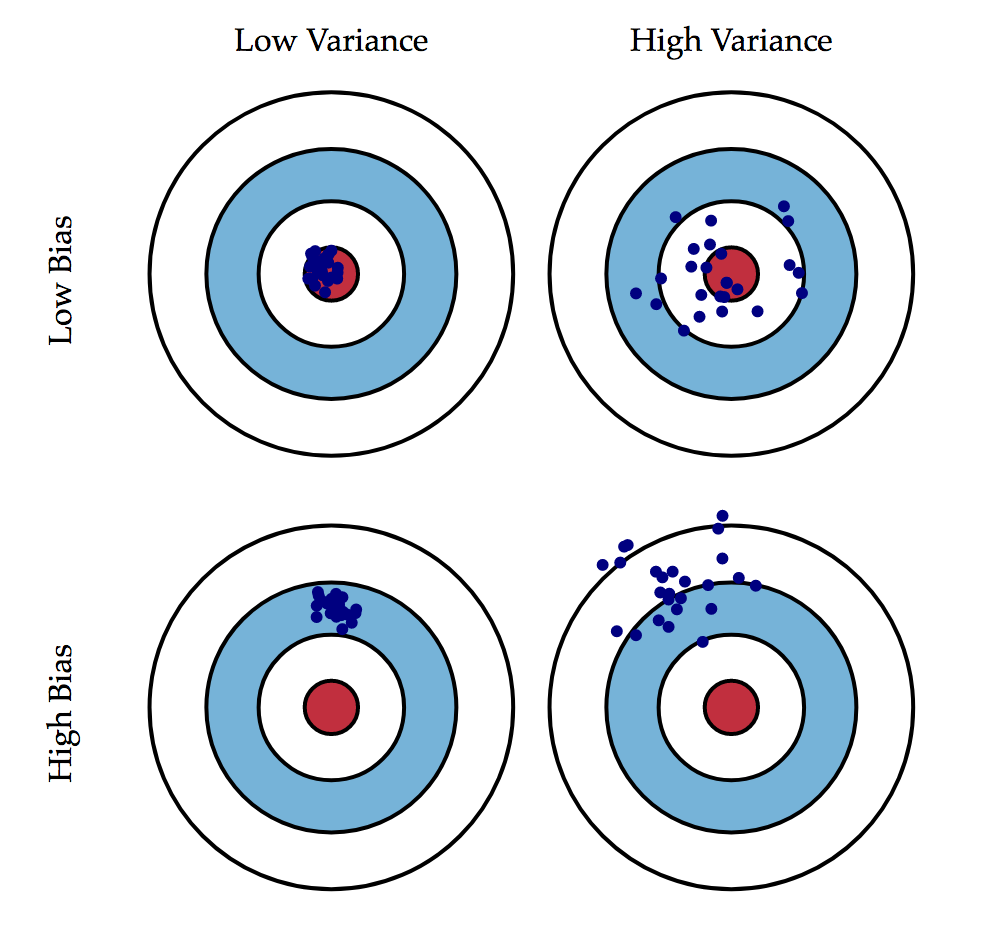
When modelling, we are trying to create a useful prediction that can help us in the future. When doing this, we have seen how we need to create a train test split in order to keep ourselves honest in tuning our model to the data itself. Another perspective on this problem of overfitting versus underfitting is the bias variance tradeoff. We can decompose the mean squared error of our models in terms of bias and variance to further investigate.

$ E[(y-\hat{f}(x)^2] = Bias(\hat{f}(x))^2 + Var(\hat{f}(x)) + \sigma^2$

$Bias(\hat{f}(x)) = E[\hat{f}(x)-f(x)]$
$Var(\hat{f}(x)) = E[\hat{f}(x)^2] - \big(E[\hat{f}(x)]\big)^2$

1. Split the data into a test and train set.

import pandas as pd
df = pd.read_excel('./movie_data_detailed_with_ols.xlsx')
def norm(col):
    minimum = col.min()
    maximum = col.max()
    return (col-minimum)/(maximum-minimum)
for col in df:
    try:
        df[col] = norm(df[col])
    except:
        pass
X = df[['budget','imdbRating','Metascore','imdbVotes']]
y = df['domgross']
df.head()

<style scoped> .dataframe tbody tr th:only-of-type { vertical-align: middle; }

.dataframe tbody tr th {
    vertical-align: top;
}

.dataframe thead th {
    text-align: right;
}

</style>

	budget	domgross	title	Response_Json	Year	imdbRating	Metascore	imdbVotes	Model
0	0.034169	0.055325	21 & Over	NaN	0.997516	0.839506	0.500000	0.384192	0.261351
1	0.182956	0.023779	Dredd 3D	NaN	0.999503	0.000000	0.000000	0.000000	0.070486
2	0.066059	0.125847	12 Years a Slave	NaN	1.000000	1.000000	1.000000	1.000000	0.704489
3	0.252847	0.183719	2 Guns	NaN	1.000000	0.827160	0.572917	0.323196	0.371052
4	0.157175	0.233625	42	NaN	1.000000	0.925926	0.645833	0.137984	0.231656

#Your code here

2. Fit a regression model to the training data.

#Your code here

import matplotlib.pyplot as plt
%matplotlib inline

2b. Plot the training predictions against the actual data. (Y_hat_train vs Y_train)

#Your code here

2c. Plot the test predictions against the actual data. (Y_hat_test vs Y_train)

#Your code here

3. Calculating Bias

Write a formula to calculate the bias of a models predictions given the actual data.
(The expected value can simply be taken as the mean or average value.)
$Bias(\hat{f}(x)) = E[\hat{f}(x)-f(x)]$

def bias():
    pass

4. Calculating Variance

Write a formula to calculate the variance of a model's predictions (or any set of data).
$Var(\hat{f}(x)) = E[\hat{f}(x)^2] - \big(E[\hat{f}(x)]\big)^2$

def variance():
    pass

5. Us your functions to calculate the bias and variance of your model. Do this seperately for the train and test sets.

#Train Set
b = None#Your code here
v = None#Your code here
#print('Bias: {} \nVariance: {}'.format(b,v))

#Test Set
b = None#Your code here
v = None#Your code here
#print('Bias: {} \nVariance: {}'.format(b,v))

6. Describe in words what these numbers can tell you.

#Your description here (this cell is formatted using markdown)

7. Overfit a new model by creating additional features by raising current features to various powers.

#Your Code here

8a. Plot your overfitted model's training predictions against the actual data.

#Your code here

8b. Calculate the bias and variance for the train set.

#Your code here

9a. Plot your overfitted model's test predictions against the actual data.

#Your code here

9b. Calculate the bias and variance for the train set.

#Your code here

10. Describe what you notice about the bias and variance statistics for your overfit model.

#Your description here (this cell is formatted using markdown)