An implementation of a Convolutional Neural Network (CNN) on a big image dataset. I used pytorch but you can use also a different deep layer framework.
The code implements a basic Neural Network (NN) and Convolutional Neural Network (CNN) with data loading, training, and evaluation (i.e. testing) phase. The training and testing are conducted on CIFAR 100 dataset (already included in Pytorch).
Note: I would recommend not using your NVIDIA card (or other) on your PC as usually it does not have a well-done Deep Learning framework setup. You could use google colab: a very user-friendly Python notebook from Google in which you can install Python packages, download datasets, plot images, and have a free GPU to do training.
Before starting make sure to add another code to your project and paste this:
!pip3 install -q http://download.pytorch.org/whl/cu90/torch-0.4.0-cp36-cp36m-linux_x86_64.whl
!pip3 install torchvision
- Neural Network Concepts
- Network Configuration Optimization
- Accuracy & Loss
- Neural Network Classes
- Resources
Every Neural Network (NN) has three types of layers: input, hidden, and output. Creating the NN architecture therefore means coming up with values for the number of layers of each type and the number of nodes in each of these layers.
For the number of neurons comprising this layer, this parameter is completely and uniquely determined once you know the shape of your training data. Specifically, the number of neurons comprising that layer is equal to the number of features (columns) in your data. Some NN configurations add one additional node for a bias term.
Every NN has exactly one output layer. Determining its size (number of neurons) is simple as it is completely determined by the chosen model configuration. If the NN is running in Machine Mode, then returns a class label (e.g., "Premium Account"/"Basic Account"); if is running in Regression Mode, then returns a value (e.g., price).
- If the NN is a regressor, then the output layer has a single node.
- If the NN is a classifier, then it also has a single node unless softmax is used in which case the output layer has one node per class label in your model.
Hidden layer
So those few rules set the number of layers and size (neurons/layer) for both the input and output layers. That leaves the hidden layers.
How many hidden layers? Well if your data is linearly separable (which you often know by the time you begin coding a NN) then you don't need any hidden layers at all. Of course, you don't need an NN to resolve your data, but it will still do the job.
Beyond that, as you probably know, there's a mountain of commentary on the question of hidden layer configuration in NNs (see the insanely thorough and insightful NN FAQ for an excellent summary of that commentary). One issue within this subject on which there is a consensus is the performance difference from adding additional hidden layers: the situations in which performance improves with a second (or third, etc.) hidden layer are very few. One hidden layer is sufficient for the large majority of problems.
So what about the size of the hidden layer(s)--how many neurons? There are some empirically-derived rules-of-thumb, of these, the most commonly relied on is 'the optimal size of the hidden layer is usually between the size of the input and size of the output layers'. Jeff Heaton, author of Introduction to Neural Networks in Java offers a few more.
In sum, for most problems, one could probably get decent performance (even without a second optimization step) by setting the hidden layer configuration using just two rules: (i) the number of hidden layers equals one, and (ii) the number of neurons in that layer is the mean of the neurons in the input and output layers.
A CNN is characterized by several parameters, such as epoch, batch size, and learning rate.
An epoch is a hyperparameter that is defined before training a model. One epoch is when an entire dataset is passed both forward and backward through the neural network only once.
One epoch is too big to feed to the computer at once. So, we divide it into several smaller batches. We use more than one epoch because passing the entire dataset through a neural network is not enough and we need to pass the full dataset multiple times to the same neural network. But since we are using a limited dataset and to optimise the learning and the graph we are using Gradient Descent which is an iterative process. So, updating the weights with a single pass or one epoch is not enough.
A batch is the total number of training examples present in a single batch and an iteration is the number of batches needed to complete one epoch.
For example: If we divide a dataset of 2000 training examples into 500 batches, then 4 iterations will complete 1 epoch.
The learning rate is one of the most important hyper-parameters to tune for training deep neural networks. If the learning rate is low, then training is more reliable, but optimization will take a lot of time because steps toward the minimum of the loss function are tiny.
If the learning rate is high, then training may not converge or even diverge. Weight changes can be so big that the optimizer overshoots the minimum and makes the loss worse.
The below diagram demonstrates the different scenarios one can fall into when configuring the learning rate.
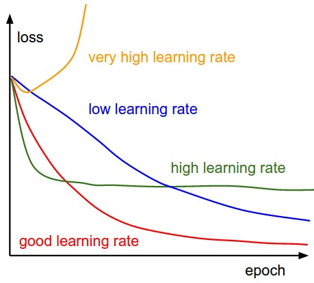
Furthermore, the learning rate affects how quickly our model can converge to local minima (aka arrive at the best accuracy). Thus getting it right from the get-go would mean less time for us to train the model.
How choose the best learning rate? If we record the learning at each iteration and plot the learning rate (log) against loss; we will see that as the learning rate increases, there will be a point where the loss stops decreasing and starts to increase. In practice, our learning rate should ideally be somewhere to the left to the lowest point of the graph.
There are a lot of things you can do to improve your NN:
- Batch normalization (at every convolutional layer): it enables the use of higher learning rates, greatly accelerating the learning process. It also enabled the training of deep neural networks with sigmoid activations that were previously deemed too difficult to train due to the vanishing gradient problem. The whole point of BN is to adjust the values before they hit the activation function, so as to avoid the vanishing gradient problem.
- Data augmentation: it is the creation of altered copies of each instance within a training dataset.
- Random horizontal flipping
- Random crop: resize to NxN and do random crop.
- Fully connected layer wider (more neurons)
- Dropout: it is a technique used to improve over-fit on neural networks, you should use Dropout along with other techniques like L2 Regularization.
- Generally, use a small dropout value of 20%-50% of neurons with 20% providing a good starting point. A probability too low has minimal effect and a value too high results in under-learning by the network.
- Use a larger network. You are likely to get better performance when dropout is used on a larger network, giving the model more of an opportunity to learn independent representations.
- Use dropout on incoming (visible) as well as hidden units. The application of dropout at each layer of the network has shown good results.
- Use a large learning rate with decay and a large momentum. Increase your learning rate by a factor of 10 to 100 and use a high momentum value of 0.9 or 0.99.
- Constrain the size of network weights. A large learning rate can result in very large network weights. Imposing a constraint on the size of network weights such as max-norm regularization with a size of 4 or 5 has been shown to improve results.
The lower the loss, the better the model (unless the model has over-fitted to the training data). The loss is calculated on training and validation and its interpretation is how well the model is doing for these two sets. Unlike accuracy, loss is not a percentage. It is a summation of the errors made for each example in training or validation sets.
In the case of neural networks, the loss is usually negative log-likelihood and residual sum of squares for classification and regression respectively. Then naturally, the main objective in a learning model is to reduce (minimize) the loss function's value for the model's parameters by changing the weight vector values through different optimization methods, such as backpropagation in neural networks.
Loss value implies how well or poorly a certain model behaves after each iteration of optimization. Ideally, one would expect the reduction of loss after each, or several, iteration(s).
The accuracy of a model is usually determined after the model parameters are learned and fixed and no learning is taking place. Then the test samples are fed to the model and the number of mistakes (zero-one loss) the model makes are recorded, after comparison to the true targets. Then the percentage of misclassification is calculated.
There are also some subtleties while reducing the loss value. For instance, you may run into the problem of over-fitting in which the model "memorizes" the training examples and becomes kind of ineffective for the test set. Over-fitting also occurs in cases where you do not employ a regularization, you have a very complex model (the number of free parameters W is large), or the number of data points N is very low.
The NN class (nn.py) is a fully connected network (multilayer perceptrons) that provides two hidden layers and one FC layer network. This class was trained on the CIFAR 100 train set.
The CNN class (cnn.py) has been trained from scratch using Stochastic gradient descent (SGD) optimizer: also known as incremental gradient descent, is an iterative method for optimizing a differentiable objective function, a stochastic approximation of gradient descent optimization. It is called stochastic because samples are selected randomly (or shuffled) instead of as a single group (as in standard gradient descent) or in the order they appear in the training set.
The number of epochs was set to 30 - the SGD optimizer needs a higher number of epochs to return the best accuracy.
Then data augmentation (i.e. RandomHorizontalFlip()) has been used to create an altered copy of each instance and improve the training.
After that, different kinds of setting parameters were tested for each used layer:
- Convolutional layer
- Kernel size
- Stride
- Padding
- Batch Normalization
- Momentum
- Affine
- Dropout
- Number of neurons
Finally, focused on the type and the number of used layers.
A pre-trained network on ImageNet and finetune it on the CIFAR 100 training set.