Turbulence Analyzer in Python

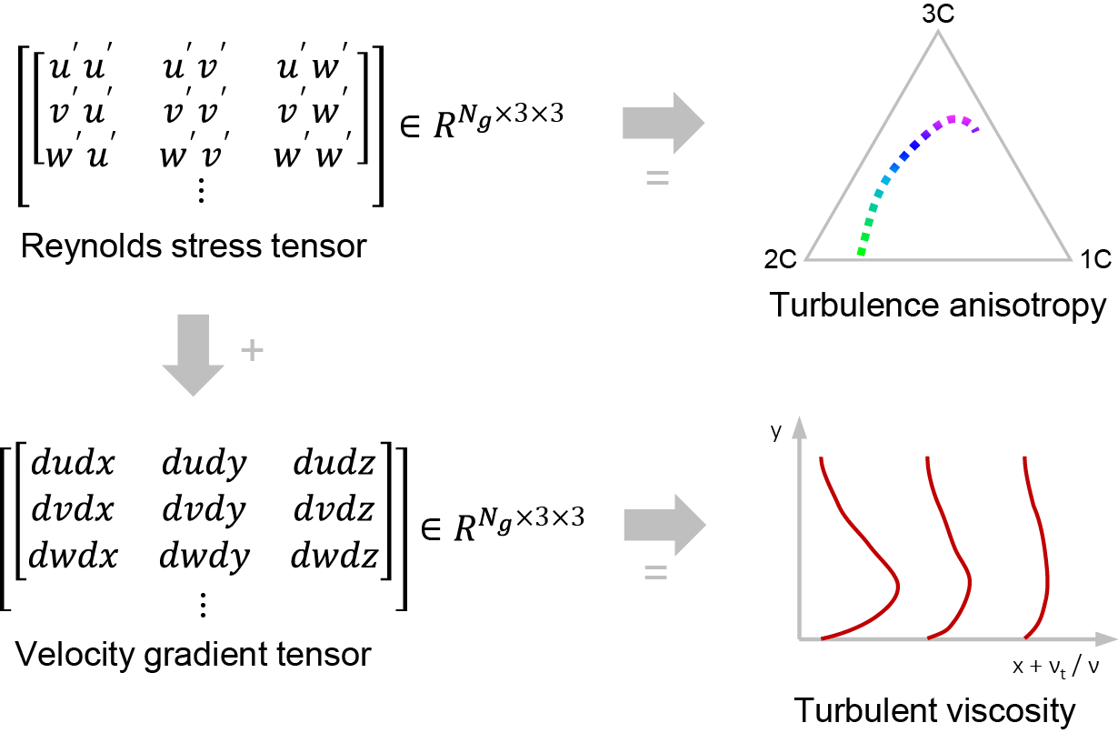
This repository contains a Python toolkit that calculates and visualizes turbulence anisotropy and turbulent viscosity from Reynolds stress components. A graphical abstract of this package is illustrated in the following figure.

If this script appears useful for your research, an explicit mention of the work [2] (for turbulence anisotropy) and [3] (for turbulent viscosity) would be highly appreciated.

Quick Start

Step 1: Download package

Download from Git clone in the terminal

git clone https://github.com/HexFluid/TurbAna.git

Download from browser

Download from this link and then unzip it.

Step 2: Install prerequisites

Launch a terminal (UNIX) or an Anaconda Prompt (Windows) window and change directory to TurbAna. Run the following command line to install/upgrade the prerequisite Python packages.

pip install -r requirements.txt

Step 3: Load example data

Run the following script with Python 3 to load the data:

import h5py
import os

current_path = os.getcwd() # assuming Python launched in the 'TurbAna' dir
data_path    = os.path.join(current_path,'tutorials','bstep_data','bstep_DNS.h5')

h5f  = h5py.File(data_path,'r')
Grid = h5f['grid'][:]         # grid point coordinates
TurbStat = h5f['TurbStat'][:] # Reynolds stress components
h5f.close()

Step 4: Calculate and visualize turbulence anisotropy

Run the following script to visualize turbulence anisotropy in the barycentric map:

import TurbAna
import matplotlib.pyplot as plt

sel_idx = (Grid[:,0]==4)&(Grid[:,1]<=1) # selected profile at x/H=4
RST = TurbAna.ReynoldsStressTensor(TurbStat[sel_idx,:]) # Reynolds stress tensor
coors = RST.BaryTriCoor() # Barycentric map coordinates: xB and yB
RGB = RST.AniRGB() # RGB color values from turbulence anisotropy eigenvalues

fig = TurbAna.plot_bary_tri()
plt.scatter(coors[:,0], coors[:,1], facecolors=RGB, zorder=0)

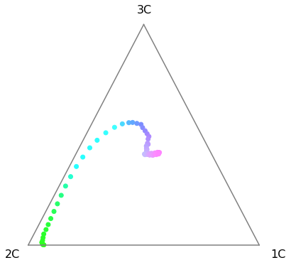
Expected results:

For more postprocess tutorials including plotting turbulence anisotropy contours and turbulent viscosity, please refer to the scripts with detailed comments in tutorials.

List of Files

.
|-- docs
|   |-- figs
|-- tutorials
|   |-- bstep_data
|   |   |-- results
|   |   |-- bstep_DDES.h5
|   |   |-- bstep_DNS.h5
|   |-- bump_data
|   |   |-- results
|   |   |-- bump_LES.h5
|   |-- cooling_data
|   |   |-- results
|   |   |-- cooling_DDES.h5
|   |-- SBLI_data
|   |   |-- results
|   |   |-- SBLI_DNS.h5
|   |-- 01_bstep.py
|   |-- 02_bump.py
|   |-- 03_cooling.py
|   |-- 04_SBLI.py
|-- LICENSE
|-- requirements.txt
|-- TurbAna.py

TurbAna.py: main script of turbulence analyzer
requirements.txt: a list of prerequisite Python libraries
LICENSE: license file
tutorials
- bstep_data
  - results: postprocess results of the backstep case
  - bstep_DDES.h5: DDES data (HDF5 format)
  - bstep_DNS.h5: DNS data (HDF5 format)
- bump_data
  - results: postprocess results of the bump case
  - bump_LES.h5: LES data (HDF5 format)
- cooling_data
  - results: postprocess results of the cooling case
  - cooling_DDES.h5: DDES data (HDF5 format)
- SBLI_data
  - results: postprocess results of the SBLI case
  - SBLI_DNS.h5: DNS data (HDF5 format)
- 01_bstep.py: tutorial script for the backward-facing step case
- 02_bump.py: tutorial script for the transonic bump case
- 03_cooling.py: tutorial script for the film cooling case
- 04_SBLI.py: tutorial script for the shock/boundary layer interaction (SBLI) case
docs
- figs: figures appeared in the markdown files

References

[1] Emory, M., & Iaccarino, G. (2014). Visualizing turbulence anisotropy in the spatial domain with componentality contours. Center for Turbulence Research Annual Research Briefs, 123-138. [link]

[2] He, X., Zhao, F., & Vahdati, M. (2022). Detached eddy simulation: recent development and application to compressor tip leakage flow. ASME Journal of Turbomachinery, 144(1), 011009. [DOI][preprint]

[3] He, X., Tan, J., Rigas, G., & Vahdati, M. (2022). On the Explainability of Machine-Learning-Assisted Turbulence Modeling for Transonic Flows. International Journal of Heat and Fluid Flow, 97, 109038. [preprint]

HexFluid / TurbAna