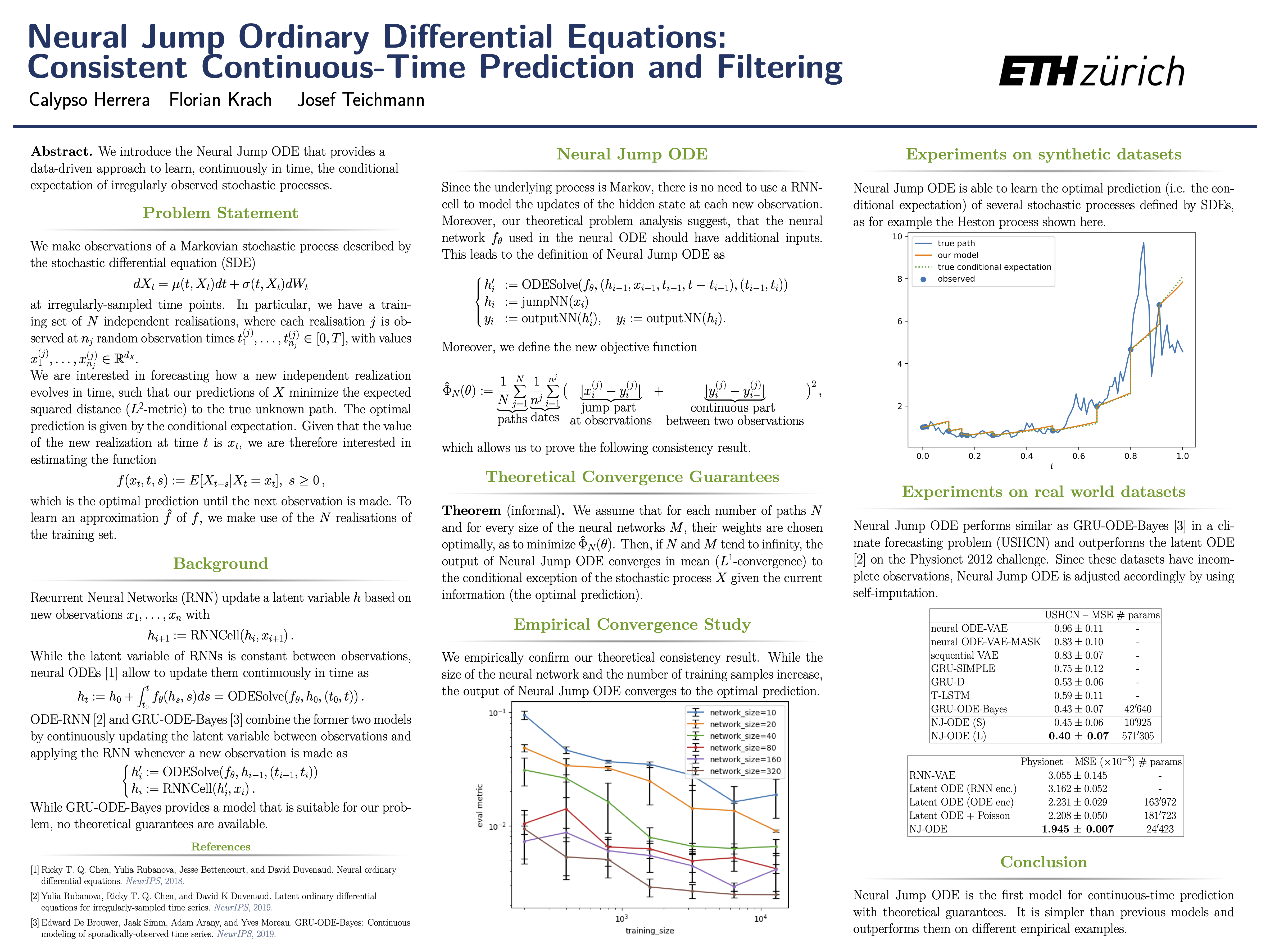
This repository is the official implementation of Neural Jump Ordinary Differential Equations: Consistent Continuous-Time Prediction and Filtering.
For a short summary of the paper see our video-presentation at the ICLR conference. Below we also provide the poster summarizing our work that we presented there.
This code was executed using Python 3.7.
To install requirements, download this Repo and cd into it. Then:
pip install -r requirements.txt
To train and test the model(s) of the paper, run these commands (other hyperparameters can be changed in the main section of demo.py):
go to the source directory:
cd NJODE
for Black-Scholes model:
python demo.py --dataset='BlackScholes'
for Heston model:
python demo.py --dataset='Heston'
for Ornstein-Uhlenbeck model:
python demo.py --dataset='OrnsteinUhlenbeck'
If no dataset for the model was generated yet, it will be generated automatically before the training starts. ATTENTION: if you run the demo for a pretrained model first, a dataset with only 100 samples (instead of 20'000) will be generated for plotting. This should be deleted before training a new model, such that a bigger dataset is generated and used.
The model is trained and concurrently saved and tested after every <save_every> epoch. The plots that are generated are saved in "../data/saved_models/id-<model_id>/plots/" and the training progress is printed.
Pre-trained models for each of the 3 stochastic models are distributed with the code and saved in "../data/saved_models/id-x" for x=1,2,3. These pre-trained models can be loaded and used to generate sample paths with the following commands:
go to the source directory:
cd controlled_ODE_RNN
- for Black-Scholes model:
python demo.py --model_id=1
- for Heston model:
python demo.py --model_id=2
- for Ornstein-Uhlenbeck model:
python demo.py --model_id=3
If no dataset for the model was generated yet, a small version of the dataset with 100 samples will be generated automatically, such that plots can be produced. ATTENTION: this dataset should be replaced with a bigger one for training (the datasets are saved in "../data/training_data/" and can be deleted there).
The pretrained models are loaded and used for plotting. No training. The plots are saved in "../data/saved_models/id-x/plots/" for x=1,2,3.
Models for the empirical convergence study were trained using parallel_train.py with the model parameters specified below
# ==========================================================================
# parallel training for convergence analysis
# ==========================================================================
in the main part of the file parallel_train.py.
For training: uncomment the code below the model params and run the file.
Models for the Heston dataset without Feller condition were trained using parallel_train.py with the model parameters specified below
# ==========================================================================
# parallel training for Heston without Feller
# ==========================================================================
in the main part of the file parallel_train.py.
For training: uncomment the code below the model params and run the file.
Models for the combined stock model dataset were trained using parallel_train.py with the model parameters specified below
# ==========================================================================
# parallel training for Combined stock models
# ==========================================================================
in the main part of the file parallel_train.py.
For training: uncomment the code below the model params and run the file.
Models for the sine stock model dataset were trained using parallel_train.py with the model parameters specified below
# ==========================================================================
# parallel training for sine stock models
# ==========================================================================
in the main part of the file parallel_train.py.
For training: uncomment the code below the model params and run the file.
Models for the comparison to GRU-ODE-Bayes were trained using parallel_train.py with the model parameters specified below
# ==========================================================================
# parallel training for GRU-ODE-Bayes
# ==========================================================================
in the main part of the file parallel_train.py.
For training: uncomment the code below the model params and run the file.
For easier evaluation after training, use the function-call:
get_training_overview(
    params_extract_desc=('dataset', "other_model",
                         'network_size', 'training_size',
                         'hidden_size', "GRU_ODE_Bayes-mixing",
                         "GRU_ODE_Bayes-logvar", "GRU_ODE_Bayes-impute",
                         "GRU_ODE_Bayes-mixing"),
    val_test_params_extract=(("max", "epoch", "epoch", "epochs_trained"),
                             ("min", "evaluation_mean_diff",
                              "evaluation_mean_diff", "eval_metric_min"),
                             ("last", "evaluation_mean_diff",
                              "evaluation_mean_diff", "eval_metric_last"),
                             ("average", "evaluation_mean_diff",
                              "evaluation_mean_diff", "eval_metric_average")
                             )
)
in extras.py.
The preprocessed climate data that was provided by GRU-ODE-Bayes together with the cross-validation indices generated with their provided code, is saved in data/training_data/climate/, s.t. models can be trained right away.
Models for cross-validation on the climate dataset were trained using parallel_train.py with the model parameters specified below
# ==========================================================================
# parallel training on climate dataset
# ==========================================================================
in the main part of the file parallel_train.py.
For training: uncomment the code below the model params and run the file.
For performing/evaluating the cross-validation use the function-call:
get_training_overview(
    params_extract_desc=('dataset', 'network_size', 'dropout_rate',
                         'hidden_size', 'data_index'),
    val_test_params_extract=(("max", "epoch", "epoch", "epochs_trained"),
                             ("min", "eval_metric",
                              "eval_metric", "eval_metric_min"),
                             ("min", "test_metric",
                              "test_metric", "test_metric_min"),
                             ("min", "eval_metric",
                              "test_metric", "test_metric_evaluation_min"),
                             ("min", "eval_loss",
                              "test_metric", "test_metric_eval_loss_min"),
                             )
)

get_climate_cross_validation(early_stop_after_epoch=100)
in extras.py.
The Physionet dataset that was used by Latent ODEs for Irregularly-Sampled Time Series is downloaded and saved automatically when training for the first time. Moreover, the preprocessing steps provided in this paper are applied automatically.
Models for validation on the Physionet dataset were trained using parallel_train.py with the model parameters specified below
# ==========================================================================
# parallel training on physionet dataset
# ==========================================================================
in the main part of the file parallel_train.py.
For training: uncomment the code below the model params and run the file.
For performing/evaluating the validation (based on 5 runs) use the function-call:
# ------------ validation of physionet training -------------
get_training_overview(
    path='{}saved_models_physionet_comparison/'.format(train.data_path),
    params_extract_desc=('dataset', 'network_size', 'dropout_rate',
                         'hidden_size', 'data_index'),
    val_test_params_extract=(("max", "epoch", "epoch", "epochs_trained"),
                             ("min", "eval_metric",
                              "eval_metric", "eval_metric_min"),
                             ("min", "eval_metric_2",
                              "eval_metric_2", "eval_metric_2_min"),
                             )
)

get_cross_validation(
    path='{}saved_models_physionet_comparison/'.format(train.data_path),
    save_path='{}saved_models_physionet_comparison/'
              'cross_val.csv'.format(train.data_path),
    param_combinations=({'network_size': 50},
                        {'network_size': 200},
                        {'network_size': 400}),
    val_test_params_extract=(("max", "epoch", "epoch", "epochs_trained"),
                             ("min", "eval_metric",
                              "eval_metric", "eval_metric_min"),
                             ("min", "eval_metric_2",
                              "eval_metric_2", "eval_metric_2_min"),
                             ("last", "eval_metric_2",
                              "eval_metric_2", "eval_metric_2_last"),
                             ("min", "train_loss",
                              "eval_metric_2", "eval_metric_2_eval_min"),
                             ),
    target_col=('eval_metric_min', 'eval_metric_2_min',
                'eval_metric_2_last', 'eval_metric_2_eval_min')
)
in extras.py.
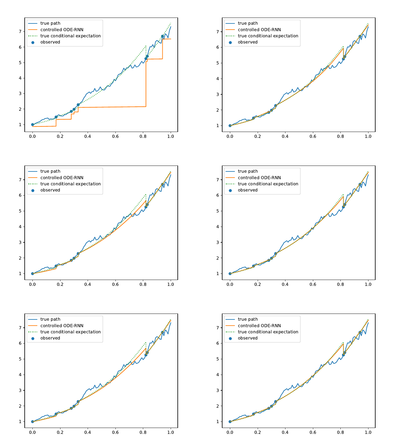
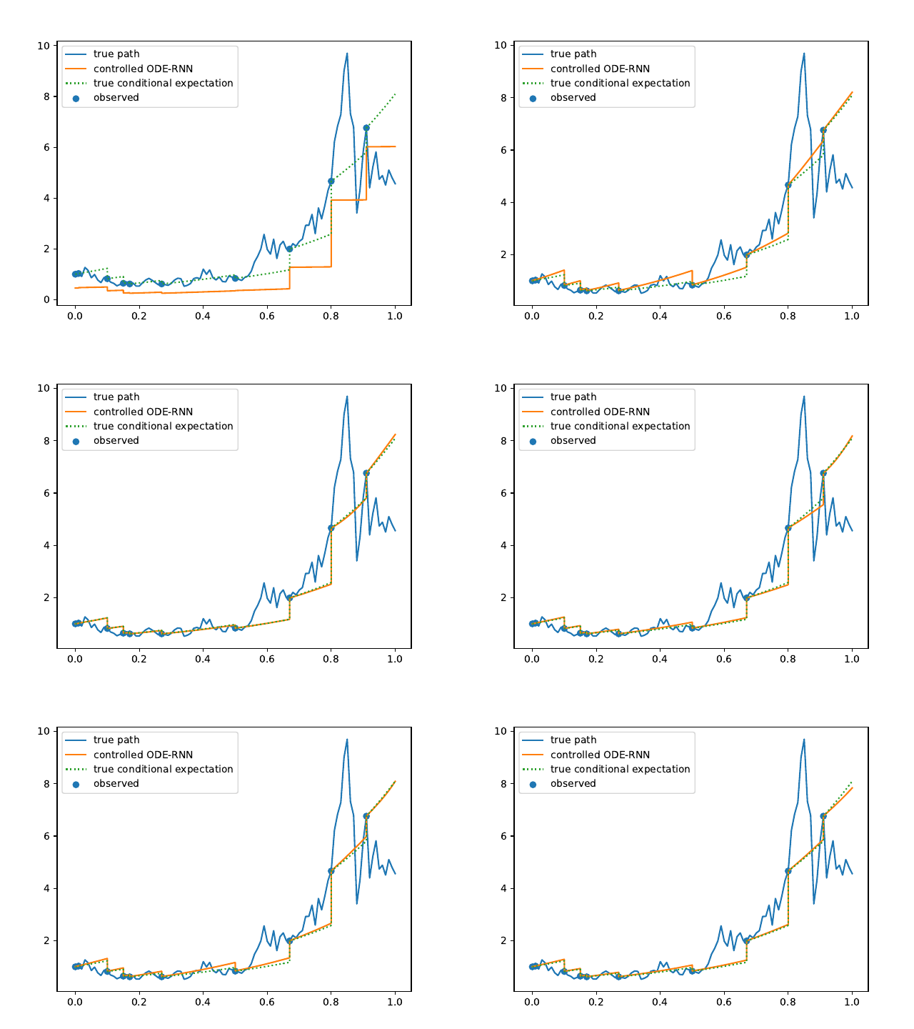
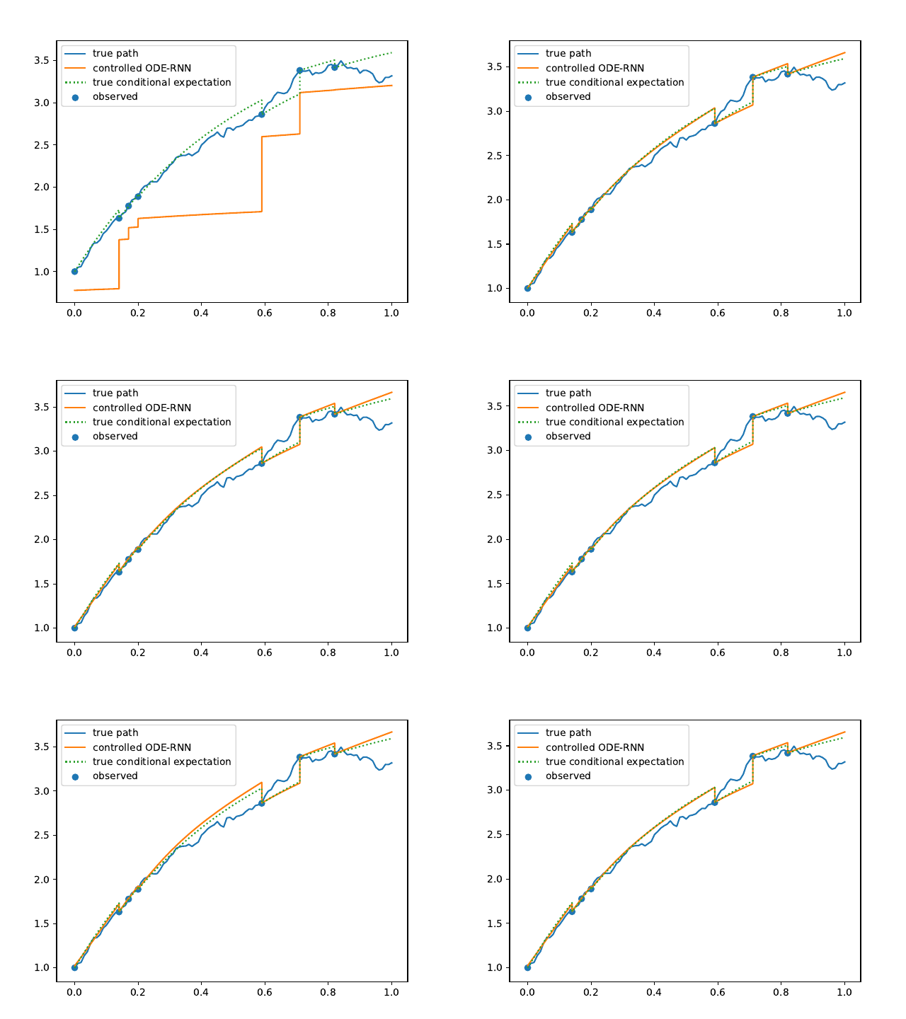
Evolution of the model output (with old name "controlled ODE-RNN") on sample test paths during training (i.e. increasing umber of epochs) for the 3 synthetic datasets.
Black-Scholes:
Heston:
Ornstein-Uhlenbeck:
This code can be used in accordance with the LICENSE.txt.
If you find this code useful, please cite our paper: Neural Jump Ordinary Differential Equations: Consistent Continuous-Time Prediction and Filtering.
@inproceedings{
herrera2021neural,
title={Neural Jump Ordinary Differential Equations: Consistent Continuous-Time Prediction and Filtering},
author={Calypso Herrera and Florian Krach and Josef Teichmann},
booktitle={International Conference on Learning Representations},
year={2021},
url={https://openreview.net/forum?id=JFKR3WqwyXR}
}
Parts of this code are based on and/or copied from the code of: https://github.com/edebrouwer/gru_ode_bayes, of the paper GRU-ODE-Bayes: Continuous modeling of sporadically-observed time series and the code of: https://github.com/YuliaRubanova/latent_ode, of the paper Latent ODEs for Irregularly-Sampled Time Series.
The GIFs of the training progress were generated with imageio:


