 A reactor neutrino simulator for Super-Kamiokande, simulating production in
reactors, oscillation to SK, cross section for IBD on free protons, and detector
smearing. Built referencing M. Baldoncini et al., "Reference worldwide model
for antineutrinos from reactors",
arXiv:1411.6475v2.
SKReact uses python 3(.7.0), it does not support python 2. Install the required modules using pip:
$ pip install -r requirements.txt.
If it is your first time running and you don't have a reactors_main.pkl file,
you can generate your own by downloading the .xls files containing reactor
information from the PRIS kindly compiled by INFN
here.
Download the "Input database" files (you will need to request the download), and
place the files into react_p/ in the SKReact directory, with their names unchanged.
Simply create the directory if it does not already exist, or change the
REACT_DIR variable in params.py if you want to pull the data from somewhere
else.
The first time running without a reactors_main.pkl file will be very slow to
start as the relevant information needs to be pulled and compiled from the
.xls files. SKReact tries to handle all inconcistencies across the files and
will print any changes in reactor information as it compiles, if you want
verbose import/import errors, change the VERBOSE_IMPORT and
VERBOSE_IMPORT_ERR values in params.py.
Running from then on with a reactors_main.pkl file will be much faster on
startup. There is a chance you will need to recompile from .xls between
SKReact releases.
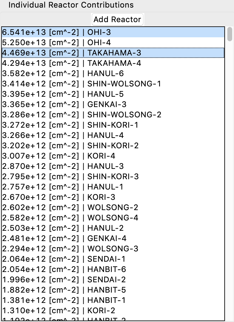
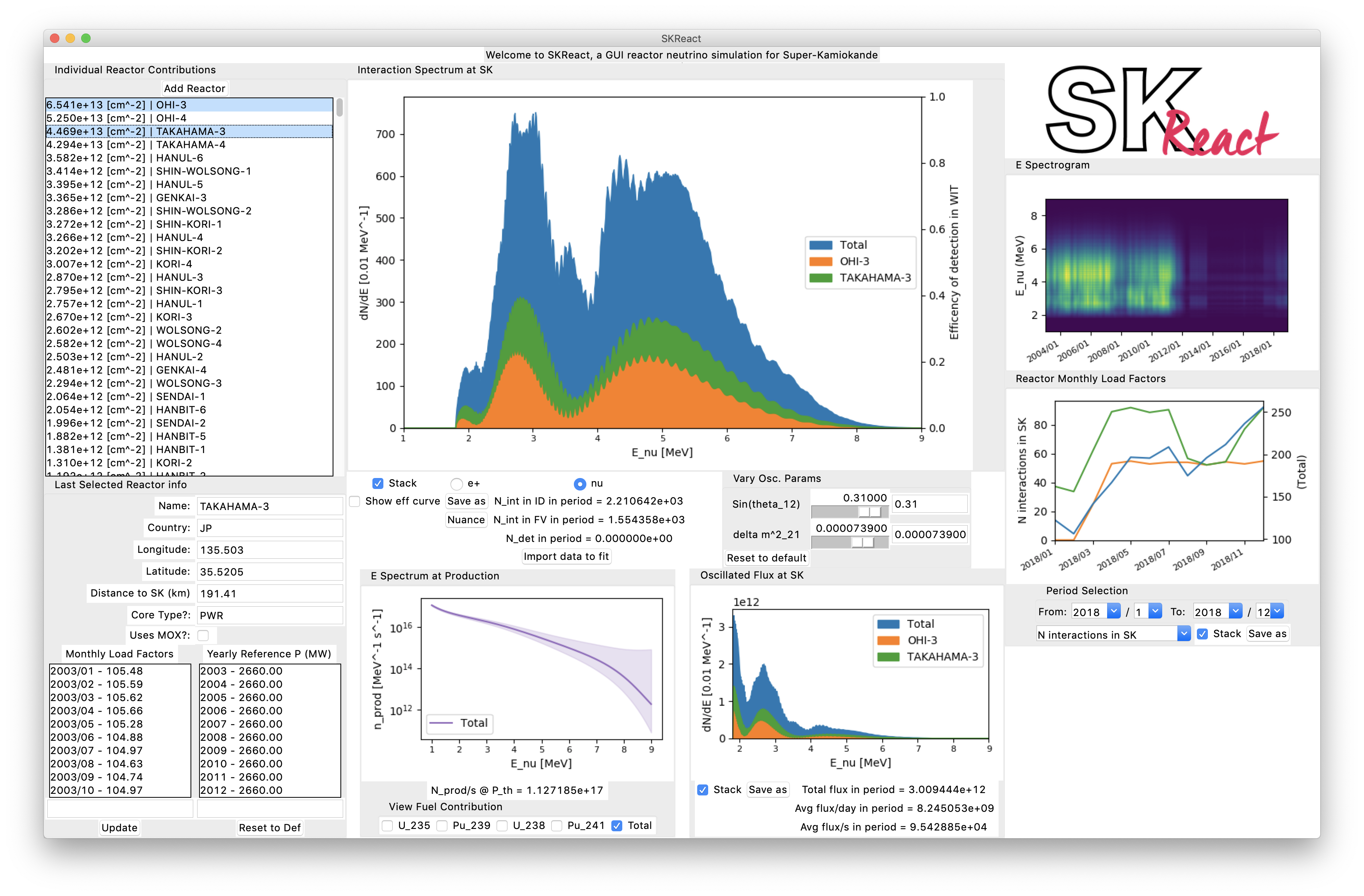
This is a list of the reactors contributing to the total spectrum at SK i.e. the reactors imported from the PRIS. It is ordered by largest flux contribution at Super-K. Select a reactor to highlight it on the spectra plots. The last selected reactor's information will appear in the reactor info pane.
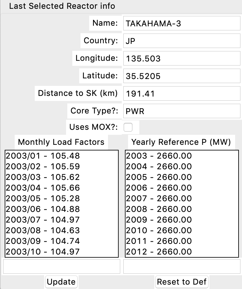
Here you can see the relevant information about the last selected reactor. You can edit the information as you like then click the Update button to re-generate the spectra.
To edit to load factor or power information, select a value in the listbox, type the desired value in the entry box below and hit return.
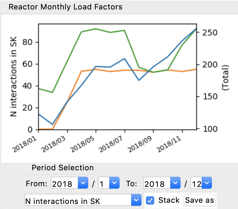
This plot lets you visualise the expected reactor signal/reactor power information, by default showing the number of interactions each month (for the total (blue) and highlighted reactors). All values dynamically update with reactor info changes except the number of interactions, which is calculated on startup. You can select the period to focus on using the drop boxes. NOTE: the selection is inclusive, i.e. the end month selected is included in the simulation, so to inspect one month, you set both start and end to the same month (will likely print errors with plotting to terminal, will be fixed in future update).
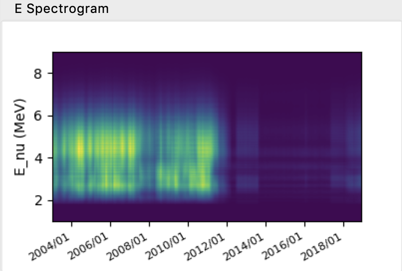
A spectrogram (calculated on startup) to visualise how the spectrum changes over time. Currently "for show" but will make more use of this in the future.
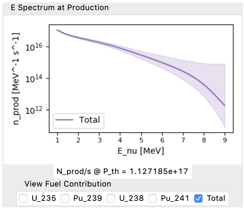
Shows the produced spectrum (/s) and n produces for the last selected reactor (varies with reactor type). Click the checkboxes to show individual fuel contributions (assumes fixed fuel fractions).
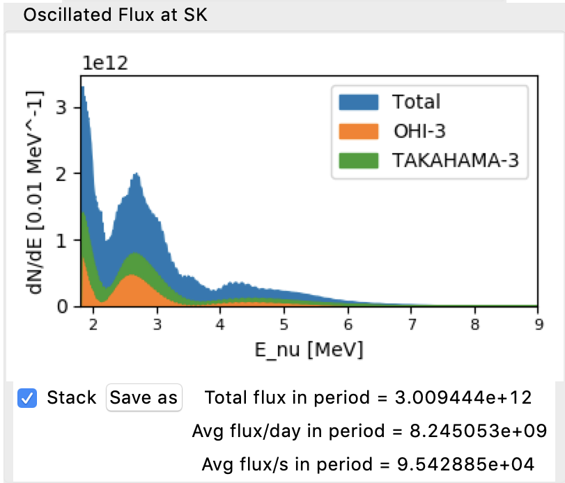
The total oscillated spectrum at SK with some numbers. Can save the plot
(with its current size, will update to produce full sized plot in future), as
well as produce a .csv of the spectrum by selecting .csv as the extension
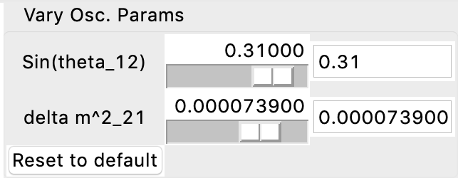
when saving. Can vary the oscillation parameters using the sliders:
This is slow (the spectra for each reactor needs to be calculated and summed on the fly), but is nice for visualising the main parameters' effects on the spectra.
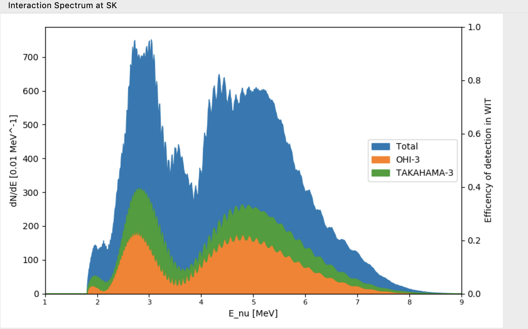
The final spectrum after multiplying the oscillated spectrum by the IBD cross section. You can view the neutrino or positron spectrum (i.e. offset by 1.806 MeV) by selecting the radio button for each in the options.
From this you can save the plot (also as .csv as with the oscillated
spectrum) or generate a .nuance file from the spectrum for input into detector
simulators (will always generate positron spectrum).
On startup, if smear_main.csv is found (change WIT_SMEAR_FILE in params.py
for other filenames) SKReact will generate a smearing matrix to multiply by the
interacted spectrum, giving a "detected" spectrum.
smear_main.csv contains the gaussian parameters for the reconstructed energy
from fixed energy in the detector and must be of the form (with headers):
e,c,mu,sig,eff
Where e is the energy reconstructed, c,mu,sig are the gaussian parameters
and eff is the efficiency of detection at that energy. You can generate this
yourself using your detector simulator by generating samples at fixed energies,
reconstructing them and fitting a gaussian. If you are an SK collaborator,
contact
alexander.goldsack@physics.ox.ac.uk for a
WIT smearing file.
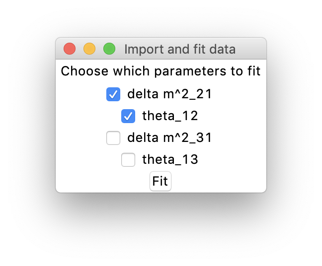
SKReact also has a (crude) fitter, which will vary selected oscillation
parameters to fit a given detected spectrum with the calculated smeared
spectrum. Click "Import data to fit" on the interacted spectrum options frame
and select a .csv file of format e,bin content (without headers). Then
select which parameters you'd like to fit, and run. The fitter cyclicly finds a
minima in a range defined under # FITTING in params.py.
NOTE: The fitter in SKReact is very crude and requires some tuning and optimisation/parallelisation.
For any issues, suggestions, enhancements or bugs, please post an issue on the repository's issues page. To contact me directly, please email alexander.goldsack@physics.ox.ac.uk, however please be aware my support for SKReact is primarily limited to my own requirements and so I will have to weigh up the time/personal usefulness for any modifications.
Please enjoy SKReact!
