ggols

Statistical modeling is an important technique to understanding relationships in data. In statistics classes, introductions to modeling often start by modeling one continuous ‘response’ variable, y, by one continuous ‘independent’ variable, x. After discussing statistical features of this simple modeling set-up, students are then often introduced to multivariate thinking in which a second explanatory variable is used in modeling; most commonly, this second variable is an cat or categorical variable, where conditions are discrete and therefore easier to reason about.

Using the popular and powerful ggplot2 library, visualizations of models with one explanatory variable is relatively straightforward via the ggplot2::geom_smooth() function. However, it is much more difficult to use the ggplot2 package to visualize models with a second, categorical prediction variable. geom_smooth will indicate different predictions for different categories when an categorical variable is included in the aesthetic specification via for example aes(linetype = my_cat) or aes(color = my_cat). However, the model estimation is performed independently for each category; geom_smooth is instructed to break each dataset apart and compute group-wise. Compelling, 2-D visuals of the models are possible, but challenging to choreograph with ggplot2.

The ggplot2 extension package {{ggols}} (from OLS) aims to provide new geom_*’s that will allow for easy visualization of models of the form y ~ x + z where x and y are continuous and z is discrete. The extension strategy that is used is to specify that model computation happen at the panel level (or maybe layer); and not the group level. In addition to providing functionality like geom smooth, which allows for easy visualization of a smear of model predictions and confidence intervals, {{ggols}} also seeks to provide functions that allow for easy visualization of other statistical quantities (like residuals, prediction interval, intercepts, etc.)

The goal of ggols is to …

Installation

You can install the released version of ggols from CRAN with:

install.packages("ggols")

And the development version from GitHub with:

# install.packages("devtools")
devtools::install_github("EvaMaeRey/ggols")

ggxmean gives us all the geom_lm_* functions

library(tidyverse)
#> ── Attaching core tidyverse packages ──────────────────────── tidyverse 2.0.0 ──
#> ✔ dplyr     1.1.0     ✔ readr     2.1.4
#> ✔ forcats   1.0.0     ✔ stringr   1.5.0
#> ✔ ggplot2   3.4.1     ✔ tibble    3.2.0
#> ✔ lubridate 1.9.2     ✔ tidyr     1.3.0
#> ✔ purrr     1.0.1     
#> ── Conflicts ────────────────────────────────────────── tidyverse_conflicts() ──
#> ✖ dplyr::filter() masks stats::filter()
#> ✖ dplyr::lag()    masks stats::lag()
#> ℹ Use the conflicted package (<http://conflicted.r-lib.org/>) to force all conflicts to become errors
library(ggxmean)

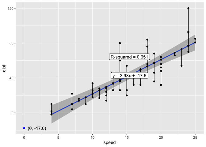
ggplot(cars) +
  aes(x = speed, y = dist,) +
  geom_point() +
  geom_lm() +
  geom_lm_intercept(color = "blue") +
  geom_lm_intercept_label(hjust = -.2) +
  geom_lm_conf_int() +
  geom_lm_residuals() +
  geom_lm_fitted() +
  geom_lm_formula() + 
  ggols:::geom_lm_rsquared() #should be moved to ggxmean

Visualization, adding cat var

library(ggols)
#> 
#> Attaching package: 'ggols'
#> The following objects are masked from 'package:ggxmean':
#> 
#>     geom_lm_cat, good_digits

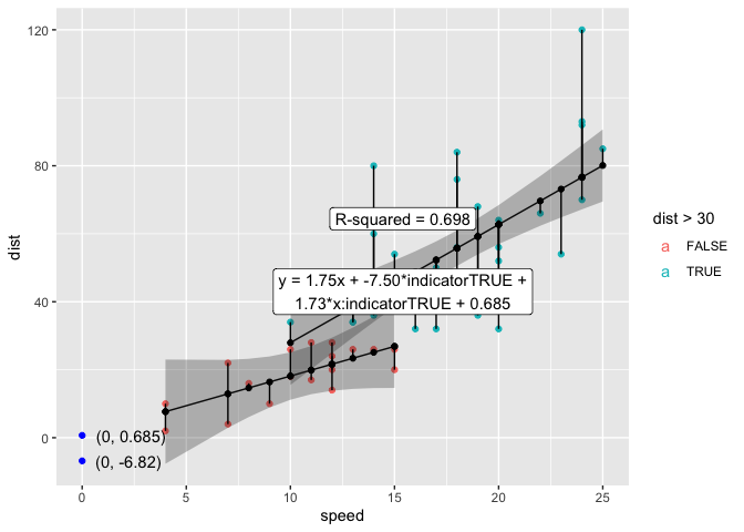
ggplot(cars) +
  aes(x = speed, y = dist, cat = dist > 30,
  color = dist > 30) +
  geom_point() +
  geom_lm_cat() +
  geom_lm_cat_intercept(color = "blue") +
  geom_lm_cat_intercept_label(hjust = -.2) +
  geom_lm_cat_conf_int() +
  geom_lm_cat_residuals() +
  geom_lm_cat_fitted() +
  geom_lm_cat_formula() +
  geom_lm_cat_rsquared()

Visualization, adding cat interaction

ggplot(cars) +
  aes(x = speed, y = dist, cat = dist > 30,
  color = dist > 30) +
  geom_point() +
  geom_lm_interaction() +
  geom_lm_interaction_intercept(color = "blue") +
  geom_lm_interaction_intercept_label(hjust = -.2) +
  geom_lm_interaction_conf_int() +
  geom_lm_interaction_residuals() +
  geom_lm_interaction_fitted() +
  geom_lm_interaction_formula() +
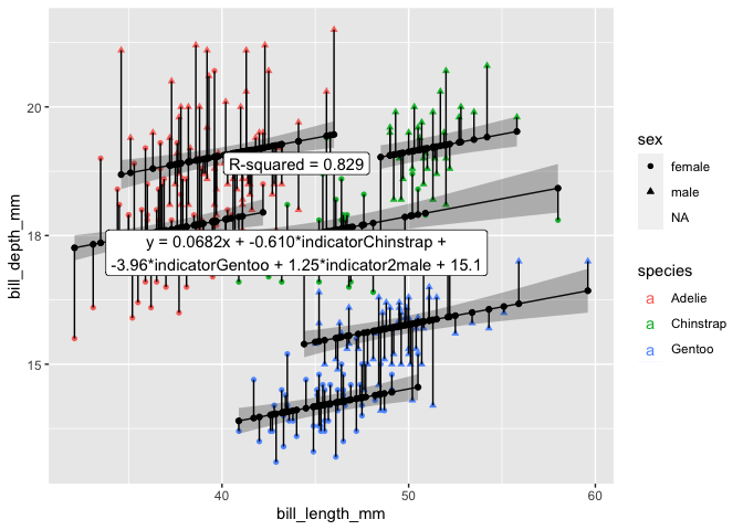
  geom_lm_interaction_rsquared()

Visualization, and two cat variables

ggplot(palmerpenguins::penguins) +
  aes(x = bill_length_mm, y = bill_depth_mm, 
      cat = species, cat2 = sex,
      color = species, shape = sex) +
  geom_point() +
  geom_lm_cat2() +
  geom_lm_cat2_conf_int() + 
  geom_lm_cat2_residuals() +
  geom_lm_cat2_fitted() +
  geom_lm_cat2_formula() +
  geom_lm_cat2_rsquared() +
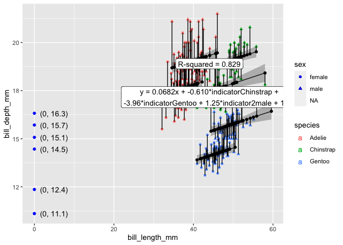
  NULL

last_plot() + 
  geom_lm_cat2_intercept(color = "blue") +
  geom_lm_cat2_intercept_label(hjust = -.2)

ggplot(palmerpenguins::penguins) +
  aes(x = bill_length_mm, y = bill_depth_mm, 
      cat = species, 
      color = species, shape = sex) +
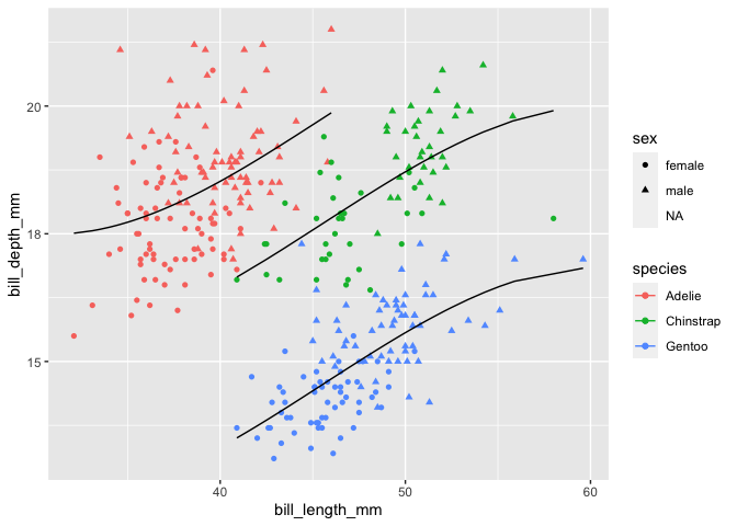
  geom_point() +
  geom_lm_cat(formula = y ~ I(x^3) + I(x^2) + x + cat)

# the implementation should change; curves expose problem. The non-smoothness shows prediction not made along parts not supported with data

EvaMaeRey / ggols