The goal of this assignment is to apply your knowledge about linear regression to a real-world problem. Your task for the next two weeks will be to analyze the given data using the techniques we have learned up to now.
Figure 0: Machine Learning explained by xkcd.com
Injection molding (Spritzgiessen) is a highly complex process. Environmental conditions, varying characteristics of the input materials, and internal machine parameters and conditions have a direct impact on the
produced components. Often the machine operator has to tune machine settings for each new part in order
to achieve an optimal performance and quality. The institutes ICOM and IWK are currently working on a
joint project with the goal to develop an automated quality assurance system for injection molding machines.
For a set of produced parts, internal machine measurements and parameters, as well as the resulting mass of
the part, have been logged. Your task will be to estimate the mass of a part, given the machine measurements.
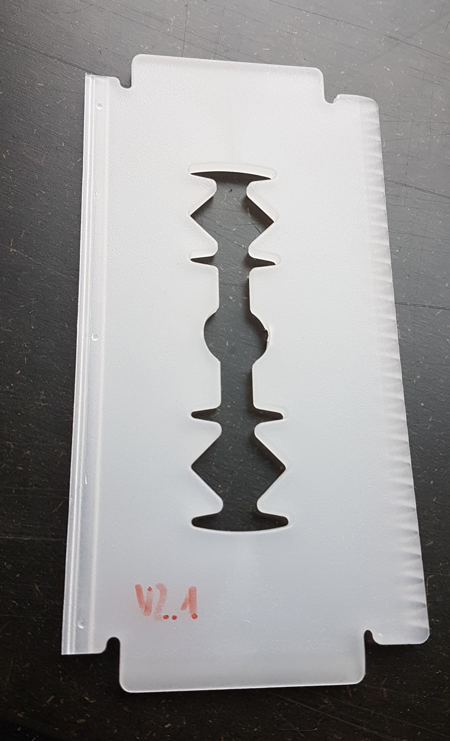
With that, the optimal amount of raw material for new parts can be found. The produced part is an ice
scraper, as shown in Figure 1.
 Figure 1: Ice scraper
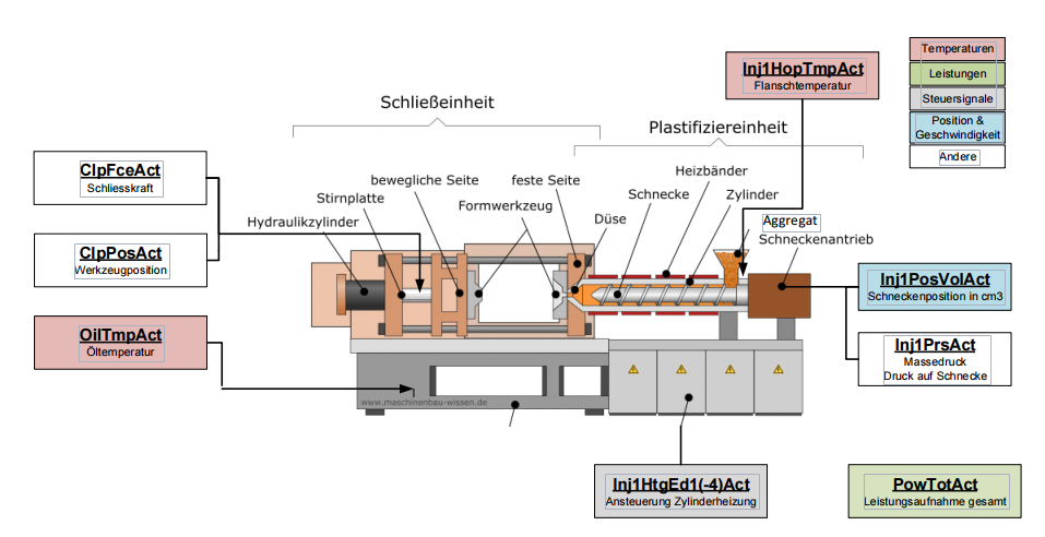
The injection molding machine with its components is shown in figure 2

The dataset consists of two CSV files: InjectionMoldingData_Train.csv, which contains all training samples, and InjectionMoldingData_Test.csv, which contains all test samples. Both files contain 9 columns: 8 predictors and the response. There are 150 training samples and 82 test samples available. All variables are described in Table 1. A drawing of a typical injection molding machine and the labels of each measurement is shown in Figure 2.
| Name | Description |
|---|---|
| PowTotAct_Min | Total power consumption of the machine |
| Inj1PosVolAct_Var | Position of the screw |
| Inj1PrsAct_meanOfInjPhase | Melt pressure on screw |
| Inj1HopTmpAct_1stPCscore | Temperature of the flange |
| Inj1HtgEd3Act_1stPCscore | Cylinder heating |
| ClpFceAct_1stPCscore | Clamping force |
| ClpPosAct_1stPCscore | Clamp position |
| OilTmp1Act_1stPCscore | Oil temperature |
| mass | Mass of the produced part |
Table 1: Description of predictors and response of the injection molding dataset.
- Analyze the training data. Is there a variable which is highly correlated to another variable? List all variables with correlation coefficients ≥ 0.9.
- Assume you can only choose one feature to predict the mass as well as possible. Which variable do you select? Explain why you select this variable and show the relevant numbers (p-value and R2 -value).
- Build a linear regression model which uses as many input variables as required. Keep in mind that each sensor costs money, so remove variables which are not needed from the model. List the selected variables and the relevant numbers for selecting them (p-value and R2 -value).
- Use the selected model to predict the mass on the test data. Compare the training MSE to the test MSE. How does your model perform on the test data?
- Add higher-order terms, such as quadratic terms or interaction terms to improve the model. Judge the model quality (R2 values). Again, compare the training MSE to the test MSE.
First, we prepare the program to read in the training data and the test data. I used panda for this and i also imported numpy for later use
import numpy as np
import pandas as pd


def main():
    training_data_input = "../data/InjectionMolding_Train.csv"
    test_data_input = "../data/InjectionMolding_Test.csv"
    training_data = pd.read_csv(training_data_input, usecols=[0, 1, 2, 3, 4, 5, 6, 7, 8])


if __name__ == '__main__':
    main()
For the correlation between variables, i decided to use the pandas correlation function
def correlate_data(data):
    corr = data.corr()
    return corr


def plot_correlation_matrix(correlation_data):
    plt.figure(figsize=(8, 8))
    plt.imshow(correlation_data, interpolation='none', aspect='auto')
    plt.title('Correlation Matrix', fontsize=18)
    plt.colorbar()
    plt.show()


# Reduce the redundant pairs and the correlation from a predictor with itself
def get_redundant_pairs(data):
    pairs_to_drop = set()
    cols = data.columns
    for i in range(0, data.shape[1]):
        for j in range(0, i+1):
            pairs_to_drop.add((cols[i], cols[j]))
    return pairs_to_drop


# Get the top five correlations between predictors, redundancy excluded
def get_top_abs_correlations(data, n=5):
    au_corr = data.corr().abs().unstack()
    labels_to_drop = get_redundant_pairs(data)
    au_corr = au_corr.drop(labels=labels_to_drop).sort_values(ascending=False)
    return au_corr[0:n]
And in the main() function, add:
correlation_data = correlate_data(training_data)
print(get_top_abs_correlations(correlation_data))
plot_correlation_matrix(correlation_data)
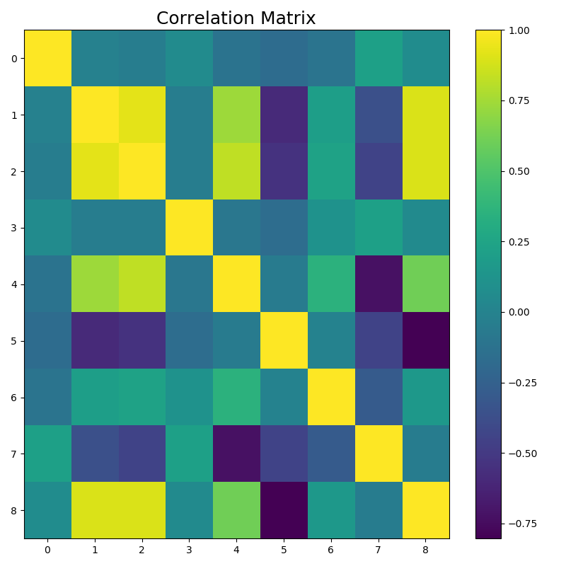
The results are a listing of the top five correlations and a plot of the correlation matrix.
Inj1PosVolAct_Var          Inj1PrsAct_meanOfInjPhase    0.995215
                           mass                         0.964210
Inj1PrsAct_meanOfInjPhase  mass                         0.944900
                           Inj1HtgEd3Act_1stPCscore     0.910607
Inj1PosVolAct_Var          Inj1HtgEd3Act_1stPCscore     0.875376
dtype: float64
Figure 3: Plotted Correlation Matrix
We have multiple pairs that correlate with more than 0.9:
Inj1PosVolAct_Var          Inj1PrsAct_meanOfInjPhase    0.995215
                           mass                         0.964210
Inj1PrsAct_meanOfInjPhase  mass                         0.944900
                           Inj1HtgEd3Act_1stPCscore     0.910607
The Position of the screw (Inj1PosVolAct_Var) correlates with Melt pressure on screw (Inj1PrsAct_meanOfInjPhase) and mass
The Melt pressure on screw (Inj1PrsAct_meanOfInjPhase) also correlates with the mass
and with the cylinder heating (Inj1HtgEd3Act_1stPCscore)
For this part of the assignment, i used the statsmodels.formula.api module to directly print a result set with all relevant information. the code looks as follows:
def statsmodel_regression(training_data, formula: str):
    model = sm.ols(formula, training_data)
    result = model.fit()
    parameters = result.summary()
    return parameters
in the main() i add the following lines
formula = "mass ~ PowTotAct_Min " \
              "+ Inj1PosVolAct_Var" \
              "+ Inj1PrsAct_meanOfInjPhase" \
              "+ Inj1HopTmpAct_1stPCscore" \
              "+ Inj1HtgEd3Act_1stPCscore" \
              "+ ClpFceAct_1stPCscore" \
              "+ ClpPosAct_1stPCscore" \
              "+ OilTmp1Act_1stPCscore"
    parameters = statsmodel_regression(training_data, formula)
    print(parameters)
The resulting table shows a lot of data.
                             OLS Regression Results
==============================================================================
Dep. Variable:                   mass   R-squared:                       0.987
Model:                            OLS   Adj. R-squared:                  0.986
Method:                 Least Squares   F-statistic:                     1312.
Date:                Wed, 23 Oct 2019   Prob (F-statistic):          2.55e-128
Time:                        13:51:36   Log-Likelihood:                 459.93
No. Observations:                 150   AIC:                            -901.9
Df Residuals:                     141   BIC:                            -874.8
Df Model:                           8
Covariance Type:            nonrobust
=============================================================================================
                                coef    std err          t      P>|t|      [0.025      0.975]
---------------------------------------------------------------------------------------------
Intercept                    30.3054      0.356     85.160      0.000      29.602      31.009
PowTotAct_Min              8.399e-07   1.06e-06      0.789      0.431   -1.26e-06    2.94e-06
Inj1PosVolAct_Var             0.0052      0.001      6.772      0.000       0.004       0.007
Inj1PrsAct_meanOfInjPhase     0.0044      0.001      7.827      0.000       0.003       0.006
Inj1HopTmpAct_1stPCscore     -0.0001      0.000     -0.309      0.758      -0.001       0.001
Inj1HtgEd3Act_1stPCscore      0.0005   4.74e-05     10.508      0.000       0.000       0.001
ClpFceAct_1stPCscore         -0.0004   4.19e-05     -9.012      0.000      -0.000      -0.000
ClpPosAct_1stPCscore         -0.0002      0.000     -1.162      0.247      -0.001       0.000
OilTmp1Act_1stPCscore         0.0014      0.000     10.888      0.000       0.001       0.002
==============================================================================
Omnibus:                       10.810   Durbin-Watson:                   2.054
Prob(Omnibus):                  0.004   Jarque-Bera (JB):               26.680
Skew:                          -0.044   Prob(JB):                     1.61e-06
Kurtosis:                       5.064   Cond. No.                     3.56e+05
==============================================================================
The R-Squared value shows, that the model explains a large portion of the variance in the response variable. The P>|t| values show significance of the predictor for the model and in general a value lower than 0.005 is preferable.
This means, that the position of the screw (Inj1PosVolAct_Var), the melt pressure of the screw (Inj1PrsAct_meanOfInjPhase), the cilinder heating (Inj1HtgEd3Act_1stPCscore), the clamp force (ClpFceAct_1stPCscore) and the oil temperature (OilTmp1Act_1stPCscore) are all viable predictors for the response.
To be able to choose the predictor with the highest R squared combined with a p-value smaller than 0,005, i add the following lines of code to the main() function
    formula = "mass ~ Inj1PosVolAct_Var"
    parameters = statsmodel_regression(training_data, formula)
    print(parameters)

    formula = "mass ~ Inj1PrsAct_meanOfInjPhase"
    parameters = statsmodel_regression(training_data, formula)
    print(parameters)

    formula = "mass ~ Inj1HtgEd3Act_1stPCscore"
    parameters = statsmodel_regression(training_data, formula)
    print(parameters)

    formula = "mass ~ ClpFceAct_1stPCscore"
    parameters = statsmodel_regression(training_data, formula)
    print(parameters)

    formula = "mass ~ OilTmp1Act_1stPCscore"
    parameters = statsmodel_regression(training_data, formula)
    print(parameters)
This results in the following output:
Parameters of position of the screw
0.80049082498907 1.1506184460940665e-53

Parameters of melt pressure of the screw
0.8098511654735854 3.2668351291332025e-55

Parameters of Cylinder heating
0.37076447406316093 1.376962458127483e-16

Parameters of clamp force
0.6463766619331468 3.1716905153677333e-35

Parameters of the oil temperature
0.0021638722385983744 0.5718968468560208
The melt pressure on the screw (Inj1PrsAct_meanOfInjPhase) has a R-squared of 0.810 and has a high correlation with the mass, so i choose this predictor.
For this model, i add the following lines of code. I went with with a forward selection process, meaning that in every iteration i add a predictor with the lowes p-value and check, if the R-squared value gets better.
 print("Add posistion of the screw to melt pressure")
    formula = "mass ~ Inj1PrsAct_meanOfInjPhase" \
              "+ Inj1PosVolAct_Var"
    model = sm.ols(formula, training_data).fit()
    print("{} {}".format(model.rsquared, model.pvalues))
    print("")

    print("Add clamp force")
    formula = "mass ~ Inj1PrsAct_meanOfInjPhase" \
              "+ Inj1PosVolAct_Var" \
              "+ ClpFceAct_1stPCscore"
    model = sm.ols(formula, training_data).fit()
    print("{} {}".format(model.rsquared, model.pvalues))
    print("")

    print("Add oil cylinder heating")
    formula = "mass ~ Inj1PrsAct_meanOfInjPhase" \
              "+ Inj1PosVolAct_Var" \
              "+ ClpFceAct_1stPCscore" \
              "+ Inj1HtgEd3Act_1stPCscore"
    model = sm.ols(formula, training_data).fit()
    print("{} {}".format(model.rsquared, model.pvalues))
    print("")

    print("Add oil temperature")
    formula = "mass ~ Inj1PrsAct_meanOfInjPhase" \
              "+ Inj1PosVolAct_Var" \
              "+ ClpFceAct_1stPCscore" \
              "+ Inj1HtgEd3Act_1stPCscore" \
              "+ OilTmp1Act_1stPCscore"
    model = sm.ols(formula, training_data).fit()
    print("{} {}".format(model.rsquared, model.pvalues))
    print("")
This procedure results in:
Add posistion of the screw to melt pressure
0.8366357970346275
Intercept                    2.138112e-58
Inj1PrsAct_meanOfInjPhase    6.251028e-08
Inj1PosVolAct_Var            2.401760e-06
dtype: float64

Add clamp force
0.9575214769385876
Intercept                    1.155154e-100
Inj1PrsAct_meanOfInjPhase     1.317330e-22
Inj1PosVolAct_Var             1.088053e-03
ClpFceAct_1stPCscore          1.511120e-44
dtype: float64

Add oil cylinder heating
0.9739211118731628
Intercept                    4.196558e-114
Inj1PrsAct_meanOfInjPhase     2.951911e-02
Inj1PosVolAct_Var             1.317246e-02
ClpFceAct_1stPCscore          4.077625e-49
Inj1HtgEd3Act_1stPCscore      4.584282e-17
dtype: float64

Add oil temperature
0.9865244378155531
Intercept                    9.643363e-126
Inj1PrsAct_meanOfInjPhase     2.753278e-14
Inj1PosVolAct_Var             7.404307e-11
ClpFceAct_1stPCscore          4.420079e-16
Inj1HtgEd3Act_1stPCscore      1.831581e-20
OilTmp1Act_1stPCscore         2.144593e-22
dtype: float64
As one can see, the first number, which is the R-squared value for the model, increases with each addition of a predictor. Also, the p-value never crosses the 0.005 line which would show a bad iteration step.
Now its time to evaluate the chosen model with the test-data. Reminder:
Formula = "mass ~ Inj1PrsAct_meanOfInjPhase"
"+ Inj1PosVolAct_Var"
"+ ClpFceAct_1stPCscore"
"+ Inj1HtgEd3Act_1stPCscore"
"+ OilTmp1Act_1stPCscore"
The mean square error is calculated as shown in the following lines of code.
# Training data Mean Squared Errors
    model = sm.ols(formula, training_data).fit()
    predictions = model.predict(training_data)
    mean_squared_error = (np.mean(np.square(training_data.mass - predictions)))
    print("Training-MSE: " + str(mean_squared_error))

    # Test data mean squared errors
    model = sm.ols(formula, training_data).fit()
    predictions = model.predict(test_data_predictors)
    mean_squared_error = np.mean(np.square(test_data_response.mass - predictions))
    print("Test-MSE: " + str(mean_squared_error))
Resulting MSE's:
Training-MSE: 0.00012927825694237846
Test-MSE: 0.00017884062549372874
Both the training and test mse's are quite low which means that on average, he predicted mass deviates from the actual mass by about 0.00018g. This is less than 0.001% deviation.
Assumption: Melt pressure interacts with other predictors.
So i test the model with the following four formulas:
mass ~ I(Inj1PrsAct_meanOfInjPhase **2) + Inj1PosVolAct_Var
mass ~ I(Inj1PrsAct_meanOfInjPhase **2) + Inj1HtgEd3Act_1stPCscore
mass ~ I(Inj1PrsAct_meanOfInjPhase **2) + ClpFceAct_1stPCscore
mass ~ I(Inj1PrsAct_meanOfInjPhase **2) + OilTmp1Act_1stPCscore Code:
formula = "mass ~ I(Inj1PrsAct_meanOfInjPhase ** 2) + Inj1PosVolAct_Var"
    model = sm.ols(formula, training_data).fit()
    print("{} \n{}".format(model.rsquared, model.pvalues))
    predictions = model.predict(test_data_predictors)
    mean_squared_error = np.mean(np.square(test_data_response.mass - predictions))
    print("Test-MSE: " + str(mean_squared_error))
    print("")

    formula = "mass ~ I(Inj1PrsAct_meanOfInjPhase ** 2) + Inj1HtgEd3Act_1stPCscore"
    model = sm.ols(formula, training_data).fit()
    print("{} \n{}".format(model.rsquared, model.pvalues))
    predictions = model.predict(test_data_predictors)
    mean_squared_error = np.mean(np.square(test_data_response.mass - predictions))
    print("Test-MSE: " + str(mean_squared_error))
    print("")

    formula = "mass ~ I(Inj1PrsAct_meanOfInjPhase ** 2) + ClpFceAct_1stPCscore"
    model = sm.ols(formula, training_data).fit()
    print("{} \n{}".format(model.rsquared, model.pvalues))
    predictions = model.predict(test_data_predictors)
    mean_squared_error = np.mean(np.square(test_data_response.mass - predictions))
    print("Test-MSE: " + str(mean_squared_error))
    print("")

    formula = "mass ~ I(Inj1PrsAct_meanOfInjPhase ** 2) + OilTmp1Act_1stPCscore"
    model = sm.ols(formula, training_data).fit()
    print("{} \n{}".format(model.rsquared, model.pvalues))
    predictions = model.predict(test_data_predictors)
    mean_squared_error = np.mean(np.square(test_data_response.mass - predictions))
    print("Test-MSE: " + str(mean_squared_error))
Result:
0.8499181662792705
Intercept                            5.687933e-60
I(Inj1PrsAct_meanOfInjPhase ** 2)    1.059112e-10
Inj1PosVolAct_Var                    7.885262e-05
dtype: float64
Test-MSE: 0.0011954647603415022

0.8812749130613108
Intercept                            2.333609e-269
I(Inj1PrsAct_meanOfInjPhase ** 2)     4.249840e-55
Inj1HtgEd3Act_1stPCscore              1.597053e-12
dtype: float64
Test-MSE: 0.000720889337867233

0.9554152188182675
Intercept                            0.000000e+00
I(Inj1PrsAct_meanOfInjPhase ** 2)    5.544314e-68
ClpFceAct_1stPCscore                 5.536850e-44
dtype: float64
Test-MSE: 0.00032245937751217455

0.9620744028690842
Intercept                             0.000000e+00
I(Inj1PrsAct_meanOfInjPhase ** 2)    2.795905e-106
OilTmp1Act_1stPCscore                 3.700602e-49
dtype: float64
Test-MSE: 0.000246656257047295
In all of the tested formulas, the R-squared is worse than the model shown and tested in section 3 and 4. The only noteworthy formula is {mass ~ I(Inj1PrsAct_meanOfInjPhase **2) + OilTmp1Act_1stPCscore} for which the R-squared is 0.962 and the MSE is 0.000247 which is remotely as good as the chosen model but still not good enough to be considered as the new model.

