Devinterview-io / dimensionality-reduction-interview-questions

🟣 Dimensionality Reduction interview questions and answers to help you prepare for your next machine learning and data science interview in 2024.

50 Must-Know Dimensionality Reduction Interview Questions

You can also find all 50 answers here 👉 Devinterview.io - Dimensionality Reduction

1. Can you define dimensionality reduction and explain its importance in machine learning?

Dimensionality reduction refers to the process of reducing the number of random variables (features) under consideration. It offers multiple advantages, such as simplifying models, improving computational efficiency, handling multicollinearity, and reducing noise.

Importance in Machine Learning

• Feature Selection: Identifying a subset of original features that best represent the data.
• Feature Engineering: Constructing new features based on existing ones.
• Visualization: Reducing data to 2D or 3D for visual inspection and interpretation.
• Computational Efficiency: Reducing computational cost, especially in high-dimensional datasets.
• Noise Reduction: Discarding noisy features.
• Collinearity Handling: Minimizing multicollinearity.
• Overfitting Mitigation: Minimizing the risk of overfitting, particularly in models with high dimensionality and small datasets.

Techniques for Dimensionality Reduction

• Feature Selection Techniques

  • Filter Methods
  • Wrapper Methods
  • Embedded Methods

• Feature Projection Techniques

  • Principal Component Analysis (PCA)
  • Linear Discriminant Analysis (LDA)
  • t-distributed Stochastic Neighbor Embedding (t-SNE)
  • Uniform Manifold Approximation and Projection (UMAP)
  • Multidimensional Scaling (MDS)
  • Autoencoders

• Hybrid Methods

  • Factor Analysis
  • Multiple Correspondence Analysis (MCA)

• Graph-Based Techniques

  • Isomap
  • Locally Linear Embedding (LLE)
  • Laplacian Eigenmaps

• Other Specialized Approaches

  • Independent Component Analysis (ICA)
  • Non-negative Matrix Factorization (NMF)

2. What are the potential issues caused by high-dimensional data?

High-dimensional data poses several challenges, often termed the "curse of dimensionality." These challenges can impact your model quality and computational efficiency.

Key Challenges

Increased Sparsity

• Issue: With higher dimensions, the available data gets distributed more sparsely, creating "empty" regions.
• Effect: This impacts the reliability of statistical estimates and machine learning predictions.

Degradation of Performance

• Issue: As sample sizes remain constant, model complexity increases with dimensionality, leading to overfitting.
• Effect: Models trained on high-dimensional data might not generalize well to new, unseen data.

Computational Overhead

• Issue: Many algorithms exhibit an "exponential curse" where computational requirements grow exponentially with the number of dimensions.
• Effect: This results in slower training, testing, and prediction times.

Difficulty in Visualizations

• Issue: Human intuition struggles to understand or interpret data in more than three dimensions.
• Effect: Insights and relationships in the data are harder to discern, hindering a thorough exploratory analysis.

Model Interpretability

• Issue: As dimensions increase, models become more complex, making it difficult to interpret the importance of each feature.
• Effect: It becomes challenging to draw clear cause-and-effect relationships between input features and model predictions.

Increased Noise

• Issue: In high-dimensional spaces, the signal-to-noise ratio can decrease, overwhelming the useful information.
• Effect: Models might mistakenly attribute significance to irrelevant or noisy features, affecting prediction accuracy.

Addressing Challenges

To mitigate the challenges of high-dimensional data, consider:

• Feature Selection: Choose a subset of relevant features to reduce sparsity, computational demands, and overfitting.
• Feature Engineering: Create new, composite features to replace or supplement high-dimensional ones.
• Dimensionality Reduction: Utilize techniques such as PCA to transform high-dimensional data into a more manageable space while preserving information.

3. Explain the concept of the "curse of dimensionality."

The curse of dimensionality refers to the numerous challenges faced when working in high-dimensional spaces, where the number of dimensions $p$ is large relative to the number of samples $n$.

Challenges of High-Dimensional Spaces

1. Sparse Data: As the $p$ increases, the data becomes sparser, requiring more data to be representative.

2. Increased Computational Demands: Many algorithms, such as $k$-means, build distance matrices, which can become excessively large and computationally intensive.

3. Degraded Model Performance: With high-dimensional spaces, models are prone to overfitting since it's easier to find variances that are just noise.

4. Increased Sensitivity to Outliers: The presence of outliers becomes more pronounced with increased dimensions.

5. Overestimation of Distance and Density: High-dimensional spaces can inflate distances between points and reduce the density of the data cloud.

6. Difficulty in Visualizing: It's challenging to visualize data beyond three dimensions. Even reducing dimensions to three or two might lead to significant loss of information.

7. Risk of Spurious Correlations: In high-dimensional space, finding false associations becomes more likely, impacting the interpretability of the model.

8. Increased Risk of Data Errors: In high-dimensional spaces, data must be especially clean and consistent. Even minor errors can have an amplified impact.

9. Unintuitive Geometry: High-dimensional spaces exhibit counterintuitive geometrical properties, leading to phenomena not observed in lower dimensions.

10. Need for Dimensionality Reduction: The limitations of high-dimensional spaces highlight the importance of undertaking dimensionality reduction whenever feasible.

4. How can dimensionality reduction prevent overfitting?

Dimensionality reduction techniques like Principal Component Analysis (PCA) can be a powerful tool for mitigating overfitting.

Mechanisms Behind Overfitting and Dimensionality Reduction

• Overfitting: Occurs when a model fits the training data too closely, capturing noise and non-representative features.
• Curse of Dimensionality: As the number of dimensions (features) increases, the number of data points required to generalize accurately grows exponentially.
• Bias-Variance Tradeoff: Models with more features can suffer from high variance (overfitting) while models with fewer features can suffer from high bias (underfitting). Striking a balance is essential.

Role of Dimensionality Reduction

• Noise Reduction: By filtering out random noise and uninformative features, dimensionality reduction helps the model focus on the most important patterns in the data.
• Smoother Decision Boundaries: Reducing the number of features often has the effect of making the classes or clusters of data points more separable or distinct in a lower-dimensional space, which in turn can lead to less convoluted decision boundaries.

Use of Cross-Validation for Model Assessment

While it is correct that proper model assessment via techniques like cross-validation is key to identifying overfitting, it's also true that dimensionality reduction techniques can help in that very process.

For example, 10-fold cross-validation is often not practical or effective in extremely high-dimensional spaces due to the curse of dimensionality. But reducing the feature space via, say, PCA, not only makes the model more interpretable and computationally efficient but also helps in more accurate model evaluation through cross-validation, as each holdout set or fold will have a better representation of the original data.

Code Example: PCA for Overfitting Mitigation

Here is the Python code:

from sklearn.model_selection import cross_val_score
from sklearn.pipeline import make_pipeline
from sklearn.preprocessing import StandardScaler
from sklearn.decomposition import PCA
from sklearn.linear_model import LogisticRegression
import numpy as np

# Creating a dataset with 100 samples and 40 features
X, y = np.random.rand(100,40), np.random.choice([0,1], 100)

# Pipeline with PCA, Standard Scaler, and Logistic Regression
clf = make_pipeline(StandardScaler(), PCA(n_components=10), LogisticRegression(max_iter=1000))

# Evaluate the model using cross-validation
accuracies = cross_val_score(clf, X, y, cv=10)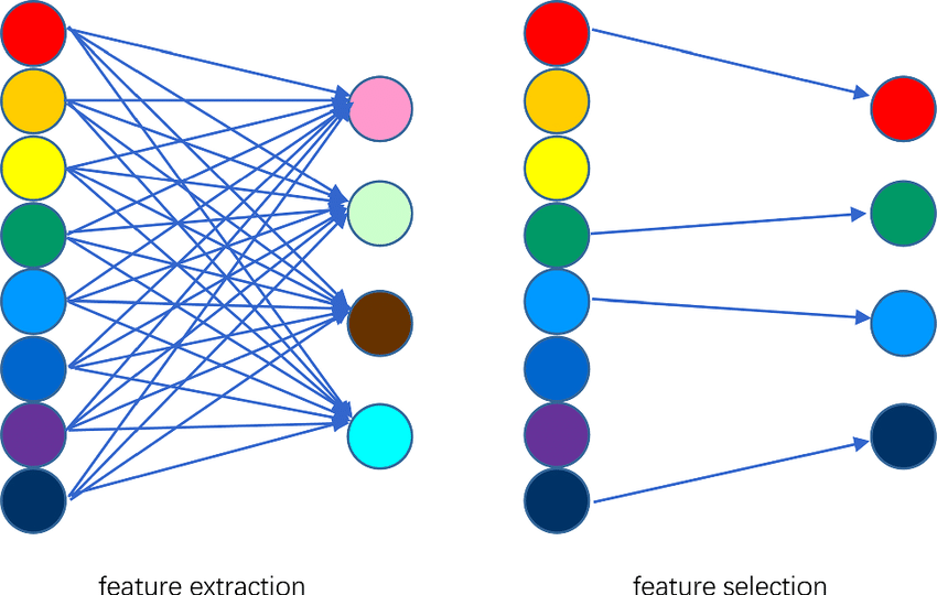
mean_accuracy = np.mean(accuracies)

5. What is feature selection, and how is it different from feature extraction?

Feature selection and feature extraction are both techniques for Dimensionality Reduction, but they approach the task in distinct ways.

Visual Representation

Key Distinctions

• Feature Selection: This method involves directly choosing a subset of the original features to be used in the model.

  This approach is preferred when variable interpretation and domain expertise are crucial. Techniques generally fall into three groups:

  • Wrapper Methods: Use predictive models to score and select features.
  • Filter Methods: Apply statistical measures to score and select features.
  • Embedded Methods: Algorithms that employ feature selection as part of the model construction.

• Feature Extraction: With this method, new a set of features, also called latent variables, are created that combine the information from the original variables.

Feature extraction is especially useful when multicollinearity among features is present or when interpretability of features is not a critical concern. Techniques in this method include:

• Principal Component Analysis (PCA)
• Linear Discriminant Analysis (LDA)
• Autoencoders

6. When would you use dimensionality reduction in the machine learning pipeline?

Dimensionality Reduction serves multiple purposes across the machine learning pipeline.

Key Functions

1. Data Preprocessing: Improves data quality and reduces training time by selecting relevant features and mitigating the curse of dimensionality.

2. Information Retention: Simplifies the understanding of the underlying structure in data. Techniques like Singular Value Decomposition (SVD), t-Distributed Stochastic Neighbor Embedding (t-SNE), and Uniform Manifold Approximation and Projection (UMAP) excel at preserving local structures in high-dimensional spaces for visual identification.

3. Noise Reduction: Filters out noisy, redundant, or irrelevant data components, leading to improved model performance.

4. Computational Efficiency: Reduces computational costs by operating on a low-dimensional space.

5. Model Interpretability: Assists in making machine learning models more interpretable and aids in understanding feature importances.

6. Overfitting Mitigation: Reduces overfitting owing to fewer spurious correlations in the data and helps models generalize better to unseen data.

7. Feature Engineering and Visualization: Utilizes the reduced feature set for improved model performance and enhanced graphical representations for interpretability.

Techniques in Dimensionality Reduction Toolbox

1. Feature Selection: Identifies a subset of relevant features. Variants include filter methods, wrapper methods like Sequential Feature Selection (SFS), and embedded methods like LASSO (Least Absolute Shrinkage and Selection Operator) regularization.

2. Feature Extraction: Transforms original features into a set of new, independent features. Examples include Principal Component Analysis (PCA) and Independent Component Analysis (ICA).

3. Manifold Learning: Focuses on characterizing the intrinsic geometry of data. Techniques such as Multi-Dimensional Scaling (MDS), t-SNE, and UMAP are common choices for visualization and clustering of high-dimensional data.

4. Autoencoders: A neural network-based approach that learns compact representations of data. Comprising an encoder for encoding information into a latent space, and a decoder for reconstructing the original input, it's effective for several machine learning tasks.

Code Example: 5 Benefits of PCA

Here is the Python code:

from sklearn.decomposition import PCA
import pandas as pd

# Create an example dataset
data = {
    'feature1': [1, 2, 3, 4, 5],
    'feature2': [5, 4, 3, 2, 1],
    'feature3': [2, 4, 6, 8, 10]
}

df = pd.DataFrame(data)

# Fit PCA to the data
pca = PCA()
pca.fit(df)

# Visualize explained variance
import matplotlib.pyplot as plt

plt.bar(range(1, 4), pca.explained_variance_ratio_, alpha=0.5, align='center')
plt.step(range(1, 4), pca.explained_variance_ratio_.cumsum(), where='mid')
plt.show()

# Transform data to reduced dimensions
reduced_data = pca.transform(df)

7. Discuss the difference between linear and nonlinear dimensionality reduction techniques.

Dimensionality Reduction: The key distinction between linear and non-linear techniques lies in their approach to unraveling complex, high-dimensional data.

Linear vs. Non-Linear Dimensionality Reduction

Key Operational Differences

• Linearity: Linear methods assume data variance, best captured in straight-line relationships. Non-linear techniques are more flexible in capturing complex, non-linear relationships.

• Optimization: Linear techniques generally entail computing eigenvectors and eigenvalues or optimizing for a projection matrix. Non-linear methods often involve searching for the most representative, lower-dimensional space, such as through graph-based structures or kernel functions.

• Computational Complexity: Linear methods can be more computationally efficient because they are essentially "parameterized" by the derived projections. In contrast, non-linear methods usually require more involved parameter-fitting processes, potentially demanding more computational resources.

• Visual Inspection: With linear methods, data can be visualized in a transformed, lower-dimensional space using simple 2D or 3D plots. Non-linear methods often need specialized tools, such as t-SNE for two-dimensional visualizations.

• Ease of Interpretation: Linear methods often result in clear, interpretable relationships between original features and reduced dimensions. The interpretability of non-linear methods can be more challenging to discern due to the complex relationships encapsulated in the lower-dimensional space.

Exclusive Techniques for Each Class

Linear Techniques

• PCA: An eigenvalue-based method that seeks orthogonal linear projections that maximize data variance in reduced dimensions.

• Linear Discriminant Analysis (LDA): It aims to uncover linear combinations of features that best separate predefined classes in classification tasks.

Non-Linear Techniques

• t-distributed Stochastic Neighbor Embedding (t-SNE): A popular manifold learning method that uses a t-distribution to model similarities in the reduced space and a Gaussian for the original space.

• Isomap: It focuses on preserving geodesic distances on a non-linear manifold, leveraging a nearest-neighbors graph to achieve this.

• Kernel PCA: An extension of PCA that employs the "kernel trick," allowing non-linear classification or regression by projecting data into a high-dimensional feature space.

• Locally Linear Embedding (LLE): Seeks to represent each data point as a linear combination of its neighbors, aiming to preserve local neighborhood structure.

• Autoencoders: Neural-network based models where the network is designed to learn an efficient representation of the data in a lower-dimensional space.

8. Can dimensionality reduction be reversed? Why or why not?

Dimensionality reduction, including methods such as Principal Component Analysis (PCA), essentially projects high-dimensional data into a lower-dimensional space. It's important to note that while the original features may not be perfectly reconstructed, the transformations applied during dimensionality reduction can still be reversed to obtain an approximation of the original data.

Mathematical Justification

The goal of PCA transforms can be mathematically defined.

Given the sample covariance matrix $S$ and an ordered set of vectors $\mathbf{u}_1, \mathbf{u}_2, \ldots, \mathbf{u}_n$ as unit eigenvectors of $S$, the transformation of a single data point, $\mathbf{x}$, into the reduced-dimensional space is:

$$ \mathbf{y} = \begin{bmatrix} u_1^T x \ u_2^T x \ \vdots \ u_m^T x \end{bmatrix} $$

where:

• $m$ is the target dimension
• $\mathbf{y}$ is the transformed or projected data

To reverse this transformation and retrieve an approximation of the original data, $\tilde{\mathbf{x}}$, the following relationship, based on the orthonormality of the $\mathbf{u}$'s is used:

$$ \begin{aligned} \mathbf{x} &\approx \tilde{\mathbf{x}} = \sum_{j=1}^{m} y_j \mathbf{u}_j \\ \end{aligned} $$

Reconstruction Levels

The original data can be approximated with the reduced-dimensional data. This approximation is an attempt to recreate the original data using fewer features and is given by:

$$ \text{Approximation}(\mathbf{x}) = \text{Projected}(\mathbf{x}) \cdot \text{Back-projected} $$

where:

• Projected is the data in the reduced-dimensional space
• Back-projected transforms the projected data back to the original feature space

Code Example: Reconstructing Transformed Data

Here is the Python code:

def approximate_original(x, y, u, m):
    """
    Reverse-transforms and reconstructs the original data, x, using the projected data, y, and the
    unit eigenvectors, u, and the target dimension, m.
    """
    back_projected = np.dot(y, u.T[:, :m])  # Undo the projection
    approximation = np.dot(back_projected, u[:, :m])  # Reconstruct the original data
    return approximation

# Example usage
approximated_data = approximate_original(x, y, u, m)
print("Approximated Data:\n", approximated_data)

Limitations of the Reversal Process

• Loss of Information: During dimensionality reduction, information is discarded. Reversing this process will never perfectly recover the original data.

• De-correlation vs. Compression: PCA aims to de-correlate data, making it more efficient to encode. It's designed to reduce redundancy, not solely dimensionality. This means reversing the transformation will retrieve a de-correlated version, but not necessarily the original.

• Bijective Nature: A bijective transformation is one that is both injective (one-to-one) and surjective (onto). It maps each point in the original space to a unique point in the target space and vice versa. PCA is injective but not surjective, meaning exact reversibility is not possible.

9. Explain Principal Component Analysis (PCA) and its objectives.

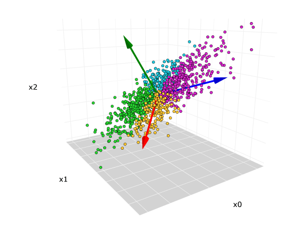
Principal Component Analysis (PCA) is a popular algorithm for dimensionality reduction and feature extraction. It's especially useful when dealing with high-dimensional data or when visualizing datasets.

Visual Representation

Key Objectives

PCA aims to achieve two primary objectives:

1. Dimensionality Reduction: Identify and project data onto a smaller set of orthogonal (uncorrelated) features, known as Principal Components (PCs), while retaining as much variance in the data as possible.

2. Data Interpretation & Visualization: Simplify data representation to enhance interpretation and visual understanding.

Core Concepts

1. Principal Components (PCs): The strongest orthogonal linear combinations of original features. These capture the most variance in the data.

2. Variance: A measure of data spread that PCA seeks to maximize in the projected space.

3. Covariance Matrix: A matrix that contains the magnitudes of relationships among original features.

Source: minitab.com

Steps of PCA

1. Standardize the Data: Ensure all features have a mean of 0 and a standard deviation of 1.

2. Compute the Covariance Matrix: This matrix represents the relationships between features and is used to compute the PCs.

3. Compute the Eigenvectors & Eigenvalues: These are derived from the covariance matrix and define the directions (eigenvectors) of the PCs and their associated variance (eigenvalues).

4. Sort Eigenvectors by Eigenvalues: This determines the order of importance of the PCs; the PCs with the highest eigenvalues are the most important in explaining data variance.

5. Select the Top $k$ Eigenvectors for Dimensionality Reduction: For most datasets, retaining 2-3 PCs is sufficient for visualization.

6. Project Data onto the Chosen Eigenvectors: This step produces transformed data, which forms the new feature space.

Code Example: PCA with Scikit-Learn

Here is the Python code:

from sklearn.decomposition import PCA
import numpy as np

# Assume X is your standardized data matrix
# Let's choose k=2 for visualization

pca = PCA(n_components=2)
X_transformed = pca.fit_transform(X)

Evaluation

• Scree Plot: A graphical tool that visualizes the explained variance by each PC, helping to determine the appropriate number of PCs to retain.

• Factor Loadings: This technique maps original features to PCs, making interpretation easier. Each feature has a weight that indicates its influence on the PC.

• Reconstruction Error: This measure helps understand the data's loss of information due to reducing dimensionality.

• Cross-Validation: Validating the performance of PCA can be essential, especially when used in conjunction with a predictive model.

Considerations and Assumptions

• Linearity: PCA assumes that data relationships are linear.

• Statistical Independence: It assumes features are independent, and if not, aims to reduce correlated features through orthogonal transformations.

• Variable Importance: PCA might spread out feature variance, making it challenging to rank the most important features, which might be crucial for certain applications.

• Optimal $k$ Selection: Determining the ideal number of PCs requires domain expertise and, potentially, the use of evaluation techniques, such as the Scree plot.

• Interpretability: Transformed features in the principal component space sometimes lose direct interpretability, especially if one uses a small number of PCs.

10. How does Linear Discriminant Analysis (LDA) differ from PCA?

Both Linear Discriminant Analysis (LDA) and Principal Component Analysis (PCA) play key roles in dimensionality reduction. However, they address different objectives and operate through distinct statistical and computational mechanisms.

Core Purpose

• LDA: Emphasizes class discrimination using features that provide the most distinct separation between classes.

• PCA: Focuses on overall data variance, aiming to preserve as much variance as possible with fewer dimensions.

Data Preprocessing

• LDA: Assumes the dataset is labeled since its core objective is to maximize class separation. As a supervised method, LDA uses class labels to guide feature transformations.

• PCA: Is unsupervised, meaning it treats all data points equally, independent of labels or groupings.

Feature Selection

• LDA: Selects or generates linear combinations of features that best differentiate between classes, improving class separation in the reduced feature space.

• PCA: Optimizes the feature combinations to account for most of the data variance, irrespective of class labels.

Dimensionality Reduction

• LDA: Reduces dimensions to a number smaller than, or equal to, $c - 1$, where $c$ is the number of classes.

• PCA: The number of retained dimensions is determined by the desired percentage of variance to preserve or through criteria like the elbow method. Typically, it reduces dimensions to a number much smaller than the original feature set.

Computational Method

• LDA: Computed based on within-class and between-class scatter matrices.

• PCA: Utilizes the covariance or correlation matrix or, in some versions, the singular value decomposition (SVD) of the data matrix.

Code Example: LDA

Here is the Python code:

from sklearn.discriminant_analysis import LinearDiscriminantAnalysis as LDA

# Assuming you have X (feature set) and y (labels)
lda = LDA(n_components=2)  # Setting number of components to 2 for visualization

X_lda = lda.fit_transform(X, y)

Code Example: PCA

Here is the Python code:

from sklearn.decomposition import PCA

pca = PCA(n_components=2)  # Reducing dimensions to 2 for visualization

X_pca = pca.fit_transform(X)

11. What is the role of eigenvectors and eigenvalues in PCA?

Principal Component Analysis (PCA) is heavily reliant on eigenvectors and eigenvalues in streamlining data while minimizing information loss.

Eigenvectors & Eigenvalues Fundamentals

• Eigenvectors are non-zero vectors that are retained within their span during linear transformations. They indicate the direction of maximum variance in the data and are denoted by $v$ in the equation: $Av = \lambda v$. Here, $A$ is a square matrix, $v$ is an eigenvector, and $\lambda$ is its corresponding eigenvalue.

• Eigenvalues represent the scaling factor by which their associated eigenvectors are stretched or compressed during the transformation.

PCA and the Covariance Matrix

PCA calculates the covariance matrix $C$ to discern the relationships between variables, where each element $c_{ij}$ details the covariance between variables $i$ and $j$.

The covariance matrix is symmetric and positive semi-definite, meaning all its eigenvalues are non-negative, and its eigenvectors are orthogonal.

1. Eigen-Decomposition of the Covariance Matrix: Through this process, PCA identifies the eigenvectors and eigenvalues of the covariance matrix, often denoted by the matrices $P$ and $\Lambda$, respectively:

$$ C = P \Lambda P^T $$

2. Eigenvectors for Rotational Changes: The eigenvectors represent the direction of maximum variance, allowing PCA to align the dataset with these vectors, thereby effecting a form of rotation.

3. Eigenvalues for Variance Magnitudes: The eigenvalues signify the variance along the corresponding eigenvector direction. PCA uses them to evaluate and rank the eigenvectors, providing guidance on the dimensions to eliminate for dimensionality reduction.

Dimensionality Reduction Process

1. Variance Contribution Assessment: PCA determines lambda scaled dataset's variance and drop low variance directions.

2. Feature Space Transformation: By incorporating the top eigenvectors with the highest eigenvalues, PCA compresses the dataset into a lower-dimensional feature space.

3. Data Reconstruction: Through a reverse transform that incorporates top principal components, the original data is reconstructed. This step aids in visualizing and grasping the transformed dataset.

Code Example: Eigenvalues and Eigenvectors in PCA

Here is the Python code:

import numpy as np
from sklearn.decomposition import PCA

# Generate sample data
np.random.seed(0)
data = np.random.randn(5, 2)

# Perform PCA
pca = PCA(n_components=1)
pca.fit(data)

# Access eigenvalues and eigenvectors
print("Eigenvalues (Variances):", pca.explained_variance_)
print("Eigenvectors (loadings):", pca.components_)

12. Describe how PCA can be used for noise reduction in data.

One of the key applications of Principal Component Analysis (PCA) is noise reduction in data, especially in the context of image or signal processing.

The Noise Reduction Problem

In observational data, noise is often present, which can be cumbersome in analysis. Let's consider an image as point of reference where the aim is to separate meaningful information, the signal, from the random distortion, the noise.

PCA Procedure for Noise Reduction

1. Decorrelate the Data:

   Principal Components $\vec{p}_i$ act as new orthogonal axes. By transforming the data to align with them, we move into a coordinate system that uncouples the original features, reducing their correlation and the potential noise influence.

2. Component Selection and Re-Projection:

   Decision on the number of principal components to retain moderates the trade-off between noise-filtering ability and signal retention.

   • A multi-step approach may involve:
     • Visualizing variance explained by components.
     • Utilizing methods like the Elbow Criterion or Cross-Validation to estimate the optimal number.

   After the retention decision, the selected components are used to reconstruct the data. Orginal input data is projected in lower dimensional space of PCA.

3. Data Reconstruction:

   The retained principal components are matched to their projections in the original dataset. By reinjecting them into the original coordinate system, and neglecting the others, we end up with a filtered version of the signal, hopefully less influenced by noise.

   Mathematically, the reconstructed data point $\hat{\vec{x}}$ can be obtained by summing the contributions of the selected principal components.

   $$ \hat{\vec{x}} = \mu + \sum_{i=1}^{k} z_i \cdot \vec{p}_i $$

   Here, $k$ is the number of components chosen and $z_i$ are those components' projections.

Code Example: Applying PCA for Noise Reduction in Images

Here is the Python code:

from sklearn.decomposition import PCA
import numpy as np
import matplotlib.pyplot as plt

# Load and flatten the image
image = plt.imread('noisy_image.png')
flattened = image.reshape((-1,3))  # Assuming RGB image

# Initialize and fit PCA
pca = PCA(n_components=2)  # For simplicity, just retaining 2 components in this example
pca.fit(flattened)

# Project data in PCA space and reconstruct
projected = pca.transform(flattened)
reconstructed = pca.inverse_transform(projected)

# For visualization, reshape and display original and reconstructed images
original_image = flattened.reshape(image.shape)
reconstructed_image = reconstructed.reshape(image.shape)

plt.subplot(1, 2, 1)
plt.imshow(original_image)
plt.title('Original Image')

plt.subplot(1, 2, 2)
plt.imshow(reconstructed_image)
plt.title('Reconstructed Image')

plt.show()

13. Explain the kernel trick in Kernel PCA and when you might use it.

Kernel PCA (kPCA) extends Principal Component Analysis with the kernel trick, converting non-linear problems into linear ones.

The Kernel Trick

In traditional PCA, we work with the covariance matrix directly, computing eigenvectors and eigenvalues. In kPCA, we use the kernel matrix ($K$), which represents the pairwise similarity between the data points under a certain transformation or kernel function $\Phi$.

$$ K = [\Phi(x_i)^T \cdot \Phi(x_j)]_{i,j} $$

This can lead to a considerably high-dimensional space, $\Phi(x)$, but kPCA allows us to perform PCA in this implicit, high-dimensional space without explicitly calculating $\Phi$ or the dot products in $K$.

Practical Considerations

• Computational Efficiency: kPCA excels at non-linear embeddings, often more efficiently than full-blown non-linear techniques like t-SNE or UMAP for large datasets.

• Hyperparameter Sensitivity: The choice of kernel and its parameters can greatly influence the results. Common kernels include RBF, polynomial, and sigmoid.

• Out-of-Sample Extension: Once trained, kPCA can embed new or unseen data points without recalculating the entire kernel matrix, making it versatile for many scenarios.

• Application in Image Recognition: kPCA can be used to extract features from high-dimensional image data for tasks such as face recognition.

Code Example: Using kPCA for Data Separation

Here is the Python code:

The task is to demonstrate kPCA applied to non-linear data.

Here is the Python code:

import numpy as np
import matplotlib.pyplot as plt
from sklearn.decomposition import KernelPCA
from sklearn.datasets import make_circles

# Generate a toy dataset
np.random.seed(0)
X, _ = make_circles(n_samples=400, factor=.3, noise=.05)

# Apply kPCA with RBF kernel
kpca = KernelPCA(kernel="rbf", gamma=10)
X_kpca = kpca.fit_transform(X)

# Visualize the data in both the original and kPCA spaces
plt.figure()
plt.subplot(1, 2, 1, aspect='equal')
plt.title('Original Space')
reds = X[_==0]
blues = X[_==1]
plt.scatter(reds[:,0], reds[:,1], c='r', marker='.')
plt.scatter(blues[:,0], blues[:,1], c='b', marker='.')

plt.subplot(1, 2, 2, aspect='equal')
plt.title('kPCA Space')
plt.scatter(X_kpca[_==0, 0], X_kpca[_==0, 1], color='r', marker='.')
plt.scatter(X_kpca[_==1, 0], X_kpca[_==1, 1], color='b', marker='.')

plt.show()

14. Discuss the concept of t-Distributed Stochastic Neighbor Embedding (t-SNE).

t-Distributed Stochastic Neighbor Embedding (t-SNE) is a dimensionality reduction technique that excels at visualizing high-dimensional data.

It initially maps data points in the high-dimensional space to corresponding points in a lower-dimensional space such as 2D or 3D. t-SNE then minimizes the discrepancies in the probability distributions of the high-dimensional and low-dimensional data.

t-SNE, in contrast to principle component analysis (PCA), is distinct in that it is non-linear and is generally more suitable for visualizing complex, non-linear dataset structures. It accomplishes this by using a Student's t-distribution instead of a Gaussian distribution.

Let's break down the mechanics behind t-SNE:

Detailed Mechanism

t-SNE constructs two probability distributions:

1. A similarity distribution in the high-dimensional space.
2. A neighborhood distribution in the low-dimensional space.

It then aligns these distributions using a technique known as stochastic neighbor embedding.

Calculating High-Dimensional Distributions

• Gaussian Kernel: t-SNE measures pairwise dissimilarities in the high-dimensional data using a Gaussian kernel, which is a function based on Euclidean distances between points. This sets proximal data points to each other.

• Conditional Probabilities: These probabilities depict the likelihood of choosing one point as a neighbor, given another point.

Minimizing Discrepancies

• Gradient Descent: t-SNE utilizes a form of gradient descent to iteratively minimize the differences between the neighborhood distribution in the low-dimensional space and the similarity distribution in the high-dimensional space.

Key Design Features

• Speed and Scalability: While t-SNE works well for moderately-sized datasets, a variant called "Fast t-SNE" improves efficiency and is more suitable for larger datasets.

• Perplexity Parameter: It impacts how the algorithm balances attention between local and global aspects of the dataset and can influence the final visual output.

Practical Use-Cases

• Visualizing Dataset Relationships: t-SNE is valuable for exploring complex datasets and potentially identifying clusters or groupings.

• Preprocessing for Supervised Learning: By visually inspecting the output, potential features or patterns that might be useful for the considered task can be revealed.

• Image Analysis: t-SNE can be used to visualize high-dimensional image data, maybe even for tasks like visualizing the layers of a deep learning network.

15. What is the difference between t-SNE and PCA for dimensionality reduction?

Principal Component Analysis (PCA) and t-Distributed Stochastic Neighbor Embedding (t-SNE) are both widely used for reducing data dimensions.

They each have unique strengths and weaknesses, making them suited for different types of tasks.

Key Differences

• Global vs. Local Structure: PCA aims to capture overall variance in the dataset, making it better for visualizing global patterns. On the other hand, t-SNE emphasizes preserving local neighbor relationships, which is beneficial when visualizing local clusters or structure.

• Data Sensitivity: t-SNE is more sensitive to the local structure and density of the data, while PCA treats all dimensions of the data equally.

• Optimization Strategies: Dimensionality reduction with PCA is achieved using a computationally efficient linear transformation. In contrast, t-SNE requires a non-convex optimization, which can be more computationally expensive.

• Dealing with Noise and Outliers: While PCA is sensitive to outliers and noise because of its global variance approach, t-SNE is more robust to such data points due to its local nature.

• Interpretability: PCA provides clear insights into the specific dimensions contributing to variance, making it easier for feature interpretation. t-SNE, while powerful in visualization, doesn't maintain this direct interpretability.

Code Example: PCA and t-SNE

Here is the Python code:

# Initialize PCA and t-SNE Models
from sklearn.decomposition import PCA
from sklearn.manifold import TSNE

pca_model = PCA(n_components=2)
tsne_model = TSNE(n_components=2)

# Fit and Transform Data
reduced_pca_data = pca_model.fit_transform(data)
reduced_tsne_data = tsne_model.fit_transform(data)

Explore all 50 answers here 👉 Devinterview.io - Dimensionality Reduction