Top 53 Binary Tree Data Structure Interview Questions

You can also find all 53 answers here 👉 Devinterview.io - Binary Tree Data Structure

1. What is a Tree Data Structure?

A tree data structure is a hierarchical collection of nodes, typically visualized with a root at the top. Trees are typically used for representing relationships, hierarchies, and facilitating efficient data operations.

Core Definitions

Node: The basic unit of a tree that contains data and may link to child nodes.
Root: The tree's topmost node; no nodes point to the root.
Parent / Child: Nodes with a direct connection; a parent points to its children.
Leaf: A node that has no children.
Edge: A link or reference from one node to another.
Depth: The level of a node, or its distance from the root.
Height: Maximum depth of any node in the tree.

Key Characteristics

Hierarchical: Organized in parent-child relationships.
Non-Sequential: Non-linear data storage ensures flexible and efficient access patterns.
Directed: Nodes are connected unidirectionally.
Acyclic: Trees do not have loops or cycles.
Diverse Node Roles: Such as root and leaf.

Visual Representation

Common Tree Variants

Binary Tree: Each node has a maximum of two children.
Binary Search Tree (BST): A binary tree where each node's left subtree has values less than the node and the right subtree has values greater.
AVL Tree: A BST that self-balances to optimize searches.
B-Tree: Commonly used in databases to enable efficient access.
Red-Black Tree: A BST that maintains balance using node coloring.
Trie: Specifically designed for efficient string operations.

Practical Applications

File Systems: Model directories and files.
AI and Decision Making: Decision trees help in evaluating possible actions.
Database Systems: Many databases use trees to index data efficiently.

Tree Traversals

Depth-First Search

Preorder: Root, Left, Right.
Inorder: Left, Root, Right (specific to binary trees).
Postorder: Left, Right, Root.

Breadth-First Search

Level Order: Traverse nodes by depth, moving from left to right.

Code Example: Binary Tree

Here is the Python code:

class Node:
    def __init__(self, data):
        self.left = None
        self.right = None
        self.data = data

# Create a tree structure
root = Node(1)
root.left, root.right = Node(2), Node(3)
root.left.left, root.right.right = Node(4), Node(5)

# Inorder traversal
def inorder_traversal(node):
    if node:
        inorder_traversal(node.left)
        print(node.data, end=' ')
        inorder_traversal(node.right)

# Expected Output: 4 2 1 3 5
print("Inorder Traversal: ")
inorder_traversal(root)

2. What is a Binary Tree?

A Binary Tree is a hierarchical structure where each node has up to two children, termed as left child and right child. Each node holds a data element and pointers to its left and right children.

Binary Tree Types

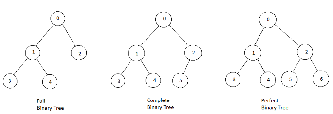
Full Binary Tree: Nodes either have two children or none.
Complete Binary Tree: Every level, except possibly the last, is completely filled, with nodes skewed to the left.
Perfect Binary Tree: All internal nodes have two children, and leaves exist on the same level.

Visual Representation

Applications

Binary Search Trees: Efficient in lookup, addition, and removal operations.
Expression Trees: Evaluate mathematical expressions.
Heap: Backbone of priority queues.
Trie: Optimized for string searches.

Code Example: Binary Tree & In-order Traversal

Here is the Python code:

class Node:
    """Binary tree node with left and right child."""
    def __init__(self, data):
        self.left = None
        self.right = None
        self.data = data

    def insert(self, data):
        """Inserts a node into the tree."""
        if data < self.data:
            if self.left is None:
                self.left = Node(data)
            else:
                self.left.insert(data)
        elif data > self.data:
            if self.right is None:
                self.right = Node(data)
            else:
                self.right.insert(data)

    def in_order_traversal(self):
        """Performs in-order traversal and returns a list of nodes."""
        nodes = []
        if self.left:
            nodes += self.left.in_order_traversal()
        nodes.append(self.data)
        if self.right:
            nodes += self.right.in_order_traversal()
        return nodes


# Example usage:
# 1. Instantiate the root of the tree
root = Node(50)

# 2. Insert nodes (This will implicitly form a Binary Search Tree for simplicity)
values_to_insert = [30, 70, 20, 40, 60, 80]
for val in values_to_insert:
    root.insert(val)

# 3. Perform in-order traversal
print(root.in_order_traversal())  # Expected Output: [20, 30, 40, 50, 60, 70, 80]

3. What is Binary Heap?

A Binary Heap is a special binary tree that satisfies the Heap Property: parent nodes are ordered relative to their children.

There are two types of binary heaps:

Min Heap: Parent nodes are less than or equal to their children.
Max Heap: Parent nodes are greater than or equal to their children.

Key Characteristics

Shape Property: A binary heap is a complete binary tree, which means all its levels are filled except the last one, which is filled from the left.
Heap Property: Nodes follow a specific order—either min heap or max heap—relative to their children.

Visual Representation

Array-Based Representation

Due to the complete binary tree structure, binary heaps are often implemented as arrays, offering both spatial efficiency and cache-friendly access patterns.

Root Element: Stored at index 0.
Child-Parent Mapping:
- Left child: (2*i) + 1
- Right child: (2*i) + 2
- Parent: (i-1) / 2

Example Array

Index:     0 1 2 3 4 5 6 7 8 9 10
Elements: 1 3 2 6 5 7 8 9 10 0 4

Advantages

Memory Efficiency: No extra pointers needed.
Cache Locality: Adjacent elements are stored closely, aiding cache efficiency.

Limitations

Array Sizing: The array size must be predefined.
Percolation: Insertions and deletions may require element swapping, adding computational overhead.

Code Example: Array-based Binary Heap Operations

Here is the Python code:

class BinaryHeap:
    def __init__(self, array):
        self.heap = array

    def get_parent_index(self, index):
        return (index - 1) // 2

    def get_left_child_index(self, index):
        return (2 * index) + 1

    def get_right_child_index(self, index):
        return (2 * index) + 2

# Example usage
heap = BinaryHeap([1, 3, 2, 6, 5, 7, 8, 9, 10, 0, 4])
parent_index = heap.get_parent_index(4)
left_child_index = heap.get_left_child_index(1)
print(f"Parent index of node at index 4: {parent_index}")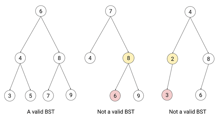
print(f"Left child index of node at index 1: {left_child_index}")

4. What is a Binary Search Tree?

A Binary Search Tree (BST) is a binary tree optimized for quick lookup, insertion, and deletion operations. A BST has the distinct property that each node's left subtree contains values smaller than the node, and its right subtree contains values larger.

Key Characteristics

Sorted Elements: Enables efficient searching and range queries.
Recursive Definition: Each node and its subtrees also form a BST.
Unique Elements: Generally, BSTs do not allow duplicates, although variations exist.

Visual Representation

Formal Properties

For any node $N$ in the BST:

$$ $$ \forall L \in \text{Left-Subtree}(N) & : \text{Value}(L) < \text{Value}(N) \\ \forall R \in \text{Right-Subtree}(N) & : \text{Value}(R) > \text{Value}(N) $$ $$

Practical Applications

Databases: Used for efficient indexing.
File Systems: Employed in OS for file indexing.
Text Editors: Powers auto-completion and suggestions.

Time Complexity

Search: $O(\log n)$ in balanced trees; $O(n)$ in skewed trees.
Insertion: Averages $O(\log n)$; worst case is $O(n)$.
Deletion: Averages $O(\log n)$; worst case is $O(n)$.

Code Example: Validating a BST

Here is the Python code:

def is_bst(node, min=float('-inf'), max=float('inf')):
    if node is None:
        return True
    if not min < node.value < max:
        return False
    return (is_bst(node.left, min, node.value) and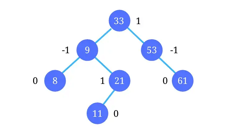
            is_bst(node.right, node.value, max))

5. What is AVL Tree? How to Balance it?

AVL Trees, named after their inventors Adelson-Velsky and Landis, are a special type of binary search tree (BST) that self-balance. This balancing optimizes time complexity for operations like search, insert, and delete to $O(\log n)$.

Balance Criterion

Each node in an AVL Tree must satisfy the following balance criterion to maintain self-balancing:

$$ \text{BalanceFactor}(N) = \text{height}(L) - \text{height}(R) \in {-1, 0, 1} $$

If a node's Balance Factor deviates from this range, the tree needs rebalancing.

This involves three steps:

Evaluate each node's balance factor.
Identify the type of imbalance: left-heavy, right-heavy, or requiring double rotation.
Perform the necessary rotations to restore balance.

Visual Representation

Types of Rotations for Rebalancing

Single Rotations

Left Rotation (LL): Useful when the right subtree is taller.
Right Rotation (RR): Used for a taller left subtree.

Double Rotations

Left-Right (LR) Rotation: Involves an initially taller left subtree.
Right-Left (RL) Rotation: Similar to LR but starts with a taller right subtree.

Code Example: AVL Operations

Here is the Python code:

class Node:
    def __init__(self, key):
        self.left = None
        self.right = None
        self.key = key
        self.height = 1

def left_rotate(z):
    y = z.right
    T2 = y.left
    y.left = z
    z.right = T2
    z.height = 1 + max(get_height(z.left), get_height(z.right))
    y.height = 1 + max(get_height(y.left), get_height(y.right))
    return y

6. What is a Red-Black Tree?

A Red-Black Tree is a self-balancing binary search tree that optimizes both search and insertion/deletion operations. It accomplishes this via a set of rules known as red-black balance, making it well-suited for practical applications.

Key Characteristics

Root: Always black.
Red Nodes: Can only have black children.
Black Depth: Every path from a node to its descendant leaves contains the same count of black nodes.

These rules ensure a balanced tree, where the longest path is no more than twice the length of the shortest one.

Benefits

Efficiency: Maintains $O(\log n)$ operations even during insertions/deletions.
Simplicity: Easier to implement than some other self-balancing trees like AVL trees.

Visual Representation

Nodes in a Red-Black Tree are visually differentiated by color. Memory-efficient implementations often use a single bit for color, with '1' for red and '0' for black.

Complexity Analysis

Time Complexity:
- Search: $O(\log n)$
- Insert/Delete: $O(\log n)$
Space Complexity: $O(n)$

Code Example: Red-Black Tree

Here is the Python code:

class Node:
    def __init__(self, val, color):
        self.left = None
        self.right = None
        self.val = val
        self.color = color  # 'R' for red, 'B' for black

class RedBlackTree:
    def __init__(self):
        self.root = None

    def insert(self, val):
        new_node = Node(val, 'R')
        if not self.root:
            self.root = new_node
            self.root.color = 'B'  # Root is always black
        else:
            self._insert_recursive(self.root, new_node)
    
    def _insert_recursive(self, root, node):
        if root.val < node.val:
            if not root.right:
                root.right = node
            else:
                self._insert_recursive(root.right, node)
        else:
            if not root.left:
                root.left = node
            else:
                self._insert_recursive(root.left, node)
        
        self._balance(node)

    def _balance(self, node):
        # Red-black balancing logic here
        pass

7. How is an AVL Tree different from a B-Tree?

Balanced search trees, such as AVL Trees and B-Trees - are designed primarily for optimized and fast search operations. However, each tree has distinct core properties and specific applications.

Key Distinctions

Structural Characteristics

AVL Trees: These are self-adjusting Binary Search Trees with nodes that can have up to two children. Balancing is achieved through rotations.
B-Trees: Multi-way trees where nodes can house multiple children, balancing is maintained via key redistribution.

Storage Optimization

AVL Trees: Best suited for in-memory operations, optimizing searches in RAM. Their efficiency dwindles in disk storage due to pointer overhead.
B-Trees: Engineered for disk-based storage, minimizing I/O operations, making them ideal for databases and extensive file systems.

Data Housing Approach

AVL Trees: Utilize dynamic memory linked via pointers, which can be more memory-intensive.
B-Trees: Data is stored in disk blocks, optimizing access by reducing disk I/O.

Search Efficiency

Both types ensure $O(\log n)$ search time. However, B-Trees often outpace AVL Trees in large datasets due to their multi-way branching.

Code Example: AVL Tree

Here is the Python code:

class Node:
    def __init__(self, value):
        self.value = value
        self.left = None
        self.right = None
        self.height = 1

class AVLTree:
    def __init__(self):
        self.root = None
    # Additional methods for insertion, deletion, and balancing.

Code Example: B-Tree

Here is the Python code:

class BTreeNode:
    def __init__(self, leaf=False):
        self.leaf = leaf
        self.keys = []
        self.child = []
    # Additional methods for operations.

class BTree:
    def __init__(self, t):
        self.root = BTreeNode(True)
        self.t = t
    # Methods for traversal, search, etc.

8. How can a Fenwick Tree (Binary Indexed Tree) be beneficial in algorithm design?

The Fenwick Tree, or Binary Indexed Tree $(BIT)$, is an extremely efficient data structure particularly suited for range queries and point updates in large sequential datasets, like arrays. Its primary strength lies in its fast update and query operations, presenting unique advantages in specific algorithmic scenarios.

Use Cases

Sum Query Efficiency: In an array, obtaining the sum of its elements up to index $i$ requires $O(n)$ time. With a BIT, this task is optimized to $O(\log n)$.
Update Efficiency: While updating an array's element at index $i$ takes $O(1)$, updating the prefix sum data to reflect this change typically needs $O(n)$ time. A BIT aids in achieving a $O(\log n)$ time update for both.
Range Queries Optimization: A BIT is helpful in scenarios where you need to frequently calculate ranges like $[l, r]$ in sequences that don't change size.

Code Example: Constructing a Binary-Indexed Tree

Here is the Python code:

def update(bit, idx, val):
    while idx < len(bit):
        bit[idx] += val
        idx += (idx & -idx)
    
def get_sum(bit, idx):
    total = 0
    while idx > 0:
        total += bit[idx]
        idx -= (idx & -idx)
    return total

def construct_bit(arr):
    bit = [0] * (len(arr) + 1)
    for i, val in enumerate(arr):
        update(bit, i + 1, val)
    return bit

To calculate the sum from index $1$ to $7$, the call is: get_sum(bit, 7) - get_sum(bit, 0). This subtractions helps in avoiding the extra point.

9. What is a Segment Tree, and how does it differ from a traditional binary tree in usage and efficiency?

Segment Trees are variant binary search trees optimized for fast range queries on an interval of a known array.

Features of a Segment Tree

Root Node: Covers the entire array or range.
Functionality: Can efficiently handle range operations like find-sum, find-max, and find-min.
Internal Nodes: Divide the array into two equal segments.
Leaves: Represent individual array elements.
Building the Tree: Done in top-down manner.
Complexity: Suitable for queries with $O(\log n)$ complexity over large inputs.
Operations: Can perform range updates in $O(\log n)$ time.

Coding Example: Range Sum Query

Here is the Python code:

class SegmentTree:
    def __init__(self, arr):
        self.tree = [None] * (4*len(arr))
        self.build_tree(arr, 0, len(arr)-1, 0)
    
    def build_tree(self, arr, start, end, pos):
        if start == end:
            self.tree[pos] = arr[start]
            return

        mid = (start + end) // 2
        self.build_tree(arr, start, mid, 2*pos+1)
        self.build_tree(arr, mid+1, end, 2*pos+2)
        self.tree[pos] = self.tree[2*pos+1] + self.tree[2*pos+2]

    def range_sum(self, q_start, q_end, start=0, end=None, pos=0):
        if end is None:
            end = len(self.tree) // 4 - 1

        if q_end < start or q_start > end:
            return 0
        if q_start <= start and q_end >= end:
            return self.tree[pos]
        mid = (start + end) // 2
        return self.range_sum(q_start, q_end, start, mid, 2*pos+1) + self.range_sum(q_start, q_end, mid+1, end, 2*pos+2)

# Example usage
arr = [1, 3, 5, 7, 9, 11]
st = SegmentTree(arr)
print(st.range_sum(1, 3))  # Output: 15 (5 + 7 + 3)

10. What is a Splay Tree, and how does its splay operation work?

The Splay Tree, a form of self-adjusting binary search tree, reshapes itself to optimize performance based on recent data access patterns. It achieves this through "splaying" operations.

Splaying Nodes

The splay operation aims to move a target node $x$ to the root position via a sequence of tree and node manipulations to increase efficiency.

The process generally involves:

Zig Step: If the node is a direct child of the root, it's rotated up.
Zig-Zig Step: If both the node and its parent are left or right children, they're both moved up.
Zig-Zag Step: If one is a left child, and the other a right child, a double rotation brings both up.

The splay sequence also ensures that descendants of $x$ remain children of $x$ after the splay operation.

Advantages and Disadvantages

Pros:
- Trees can adapt to access patterns, making it an ideal data structure for both search and insert operations in practice.
- It can outperform other tree structures in some cases due to its adaptive nature.
Cons:
- The splay operation is complex and can be time-consuming.
- Splay trees do not guarantee the best time complexity for search operations, which can be an issue in performance-critical applications where a consistent time is required.
Average Time Complexity:
- Search: $O(\log{n})$ on average.
- Insertion and Deletion: $O(\log{n})$ on average.

Code Example: Splay Tree and Splaying Operation

Here is the Python code:

class Node:
    def __init__(self, key):
        self.left = self.right = None
        self.key = key

class SplayTree:
    def __init__(self):
        self.root = None

    def splay(self, key):
        if self.root is None or key == self.root.key:
            return  # No need to splay
        dummy = Node(None)  # Create a dummy node
        left, right, self.root.left, self.root.right = dummy, dummy, dummy, dummy
        while True:
            if key < self.root.key:
                if self.root.left is None or key < self.root.left.key:
                    break
                self.root.left, self.root, right.left = right.left, self.root.left, self.root
                right, self.root = self.root, right
            if key > self.root.key:
                if self.root.right is None or key > self.root.right.key:
                    break
                self.root.right, self.root, left.right = left.right, self.root.right, self.root
                left, self.root = self.root, left
        left.right, right.left = self.root.left, self.root.right
        self.root.left, self.root.right = left, right
        self.root = dummy.right

# Splay the node with key 6
splayTree = SplayTree()
splayTree.root = Node(10)
splayTree.root.left = Node(5)
splayTree.root.left.left = Node(3)
splayTree.root.left.right = Node(7)
splayTree.root.right = Node(15)
splayTree.splay(6)

11. Explain the concept and structure of a Ternary Tree.

Ternary Trees, a type of multiway tree, were traditionally used for disk storage. They can be visualized as full or complete. Modern applications are more algorithmic than storage based. While not as common as binary trees, they are rich in learning opportunities.

Structure

Each node in a ternary tree typically has three children:

Left
Middle
Right

This organizational layout is especially effective for representing certain types of data or solving specific problems. For instance, ternary trees are optimal when dealing with scenarios that have three distinct outcomes at a decision point.

Code Example: Ternary Tree Node

Here is the Python code:

class TernaryNode:
    def __init__(self, data, left=None, middle=None, right=None):
        self.data = data
        self.left = left
        self.middle = middle
        self.right = right

12. Describe a Lazy Segment Tree and when it is used over a regular Segment Tree.

The Lazy Segment Tree supplements the standard Segment Tree by allowing delayed updates, making it best suited for the Range Update and Point Query type tasks. It is more efficient in such scenarios, especially when dealing with a large number of updates.

Lazy Propagation Mechanism

The Lazy Segment Tree keeps track of pending updates on a range of elements using a separate array or data structure.

When a range update is issued, rather than carrying out the immediate actions for all elements in that range, the tree schedules the update to be executed when required.

The next time an element within that range is accessed (such as during a range query or point update), the tree first ensures that any pending updates get propagated to the concerned range. This propagation mechanism avoids redundant update operations, achieving time complexity of $O(\log n)$ for range updates, range queries, and point updates.

Code Example: Lazy Segment Tree

Here is the Python code:

class LazySegmentTree:
    def __init__(self, arr):
        self.size = len(arr)
        self.tree = [0] * (4 * self.size)
        self.lazy = [0] * (4 * self.size)
        self.construct_tree(arr, 0, self.size-1, 0)
    
    def update_range(self, start, end, value):
        self.update_range_util(0, 0, self.size-1, start, end, value)
    
    def range_query(self, start, end):
        return self.range_query_util(0, 0, self.size-1, start, end)

    # Implement the rest of the methods

    def construct_tree(self, arr, start, end, pos):
        if start == end:
            self.tree[pos] = arr[start]
        else:
            mid = (start + end) // 2
            self.tree[pos] = self.construct_tree(arr, start, mid, 2*pos+1) + self.construct_tree(arr, mid+1, end, 2*pos+2)
        return self.tree[pos]

    def update_range_util(self, pos, start, end, range_start, range_end, value):
        if self.lazy[pos] != 0:
            self.tree[pos] += (end - start + 1) * self.lazy[pos]
            if start != end:
                self.lazy[2*pos+1] += self.lazy[pos]
                self.lazy[2*pos+2] += self.lazy[pos]
            self.lazy[pos] = 0

        if start > end or start > range_end or end < range_start:
            return

        if start >= range_start and end <= range_end:
            self.tree[pos] += (end - start + 1) * value
            if start != end:
                self.lazy[2*pos+1] += value
                self.lazy[2*pos+2] += value
            return

        mid = (start+end) // 2
        self.update_range_util(2*pos+1, start, mid, range_start, range_end, value)
        self.update_range_util(2*pos+2, mid+1, end, range_start, range_end, value)
        self.tree[pos] = self.tree[2*pos+1] + self.tree[2*pos+2]

    def range_query_util(self, pos, start, end, range_start, range_end):
        if self.lazy[pos]:
            self.tree[pos] += (end - start + 1) * self.lazy[pos]
            if start != end:
                self.lazy[2*pos+1] += self.lazy[pos]
                self.lazy[2*pos+2] += self.lazy[pos]
            self.lazy[pos] = 0

        if start > end or start > range_end or end < range_start:
            return 0

        if start >= range_start and end <= range_end:
            return self.tree[pos]

        mid = (start + end) // 2
        return self.range_query_util(2*pos+1, start, mid, range_start, range_end) + self.range_query_util(2*pos+2, mid+1, end, range_start, range_end)

13. What is a Treap, and how does it combine the properties of a binary search tree and a heap?

A Treap, also known as a Cartesian Tree, is a specialized binary search tree that maintains a dual structure, inheriting characteristics from both a Binary Search Tree (BST) and a Heap.

Core Properties

BST Order: Every node satisfies the order: $\text{node.left} < \text{node} < \text{node.right}$ based on a specific attribute. Traditionally, it's the node's numerical key-value that is used for this ordering.
Heap Priority: Each node conforms to the "parent" property, where its heap priority is determined by an attribute independent of the BST order. This attribute is often referred to as the node's "priority".

Link between Priority and Order

The priority attribute of a Treap node acts as a "tether" or a link that ensures the tree's structure conforms to both BST and heap properties. When nodes are inserted or their keys are updated in a Treap, their priorities are adjusted to maintain both of these properties simultaneously.

Operations

Insert Operation

When a new node is inserted into the Treap, both BST and heap properties are simultaneously maintained by adjusting the node's priority based on its key.

The node is first inserted based on the BST property (overriding its priority if necessary).
Then, it "percolates" up the tree based on its priority to regain the heap characteristic.

Delete Operation

Deletion, as always, is a two-step process:

Locate the node to be deleted.
Replace it with either the left or right child to keep the BST property. The replacement is specifically chosen to preserve the overall priority order of the tree.

Complexity Analysis

Time Complexity: All primary operations such as Insert, Delete, and Search take $\mathcal{O}(\log n)$ expected time.
Space Complexity: The structure preserves both BST and heap requirements with each node carrying two data attributes (key and priority).

14. What is a Balanced Tree?

A Balanced Tree ensures that the Balance Factor—the height difference between left and right subtrees of any node—doesn't exceed one. This property guarantees efficient $O(\log n)$ time complexity for search, insertion, and deletion operations.

Balanced Tree Criteria

Height Difference: Each node's subtrees differ in height by at most one.
Recursive Balance: Both subtrees of every node are balanced.

Benefits

Efficiency: Avoids the $O(n)$ degradation seen in unbalanced trees.
Predictability: Provides stable performance, essential for real-time applications.

Visual Comparison

The balanced tree maintains $O(\log n)$ height, while the unbalanced tree could degenerate into a linked list with $O(n)$ height.

Code Example: Balance Verification

Here is the Python code:

class Node:
    def __init__(self, data):
        self.data = data
        self.left = None
        self.right = None

def is_balanced(root):
    if root is None:
        return True

    left_height = get_height(root.left)
    right_height = get_height(root.right)

    return abs(left_height - right_height) <= 1 and is_balanced(root.left) and is_balanced(root.right)

def get_height(node):
    if node is None:
        return 0

    return 1 + max(get_height(node.left), get_height(node.right))

15. What are advantages and disadvantages of BST?

The Binary Search Tree (BST) is a versatile data structure that offers many benefits but also comes with limitations.

Advantages of Using BSTs

Quick Search Operations: A balanced BST can perform search operations in $O(\log n)$ time, making it much faster than linear structures like arrays and linked lists.
Dynamic Allocation: Unlike arrays that require pre-defined sizes, BSTs are dynamic in nature, adapting to data as it comes in. This results in better space utilization.
Space Efficiency: With $O(n)$ space requirements, BSTs are often more memory-efficient than other structures like hash tables, especially in memory-sensitive applications.
Versatile Operations: Beyond simple insertions and deletions, BSTs excel in:
- Range queries
- Nearest smaller or larger element searches
- Different types of tree traversals (in-order, pre-order, post-order)
Inherent Sorting: BSTs naturally keep their elements sorted, making them ideal for tasks that require efficient and frequent sorting.
Predictable Efficiency: Unlike hash tables, which can have unpredictable worst-case scenarios, a balanced BST maintains consistent $O(\log n)$ performance.
Practical Utility: BSTs find applications in:
- Database indexing for quick data retrieval
- Efficient file searching in operating systems
- Task scheduling based on priorities

Disadvantages of Using BSTs

Limited Direct Access: While operations like insert, delete, and lookup are efficient, direct access to elements by index can be slow, taking $O(n)$ time in unbalanced trees.
Risk of Imbalance: If not managed carefully, a BST can become unbalanced, resembling a linked list and losing its efficiency advantages.
Memory Costs: Each node in a BST requires additional memory for two child pointers, which could be a concern in memory-constrained environments.
Complex Self-Balancing Algorithms: While self-balancing trees like AVL or Red-Black trees mitigate the risk of imbalance, they are more complex to implement.
Lack of Global Optimum: BSTs do not readily provide access to the smallest or largest element, unlike data structures like heaps.

Explore all 53 answers here 👉 Devinterview.io - Binary Tree Data Structure