This function uses ggplot to make a surface map to visualize ocean science data. It is not suitable for terrestrial data because the land map is plotted above the data points. Land map data is contained in the package mapdata. Ocean bathymetry is optionally plotted and data is retrieved from NOAA with a call to marmap::getNOAA.bathy(); alternatively, bathymetry data can be supplied as an existing object of class bathy.
bathymetry = FALSE – can be logical (i.e. should a bathymetry be plotted) or the name of an object of class bathy
keep = FALSE – keep downloaded bathymetry in the current wd? only relevant with bathymetry=TRUE
lon.min, lon.max, lat.min, lat.max – map limits, if not supplied the range of lats and lons will be slightly extended
lats, lons – latitude and longitude of data
values – optional, data values
value.name – optional, name for the data legend
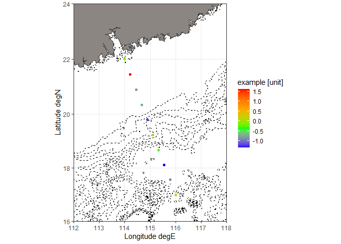
normal plot
p1 <- plot_map(
    bathymetry = TRUE,
    keep = FALSE,
    lon.min = 112,
    lon.max = 118,
    lat.min = 16,
    lat.max = 24,
    lats = seq(22, 17, length.out = 10),
    lons = seq(114, 116, length.out = 10),
    values = rnorm(10),
    value.name = "example [unit]"
)
## Registered S3 methods overwritten by 'adehabitatMA':
## method from
## print.SpatialPixelsDataFrame sp
## print.SpatialPixels sp
## Querying NOAA database ...
## This may take seconds to minutes, depending on grid size
## Building bathy matrix ...
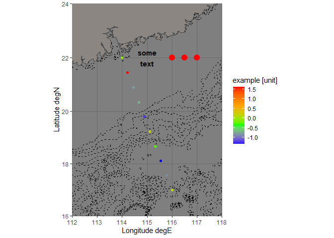
p1because the result is a ggplot, it can be extended with additional layers, and the theme can be changed
p1 +
    annotate("text", x = 115, y = 22, label = "some\ntext", size = 4, fontface = "bold") +
    geom_point(aes(x = c(116, 116.5, 117), y = c(22, 22, 22)), col = "red", size = 4) +
    theme_dark()
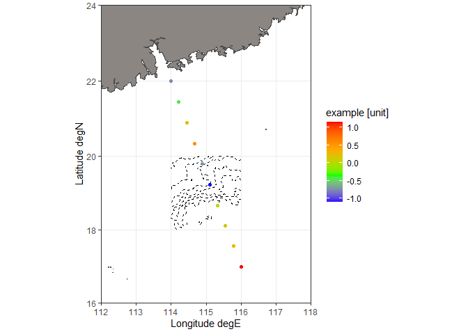
plot with bathy object supplied
plot_map(
    bathymetry = marmap::getNOAA.bathy(lon1 = 114, lon2 = 116, lat1 = 18, lat2 = 20, resolution = 1),
    keep = FALSE,
    lon.min = 112,
    lon.max = 118,
    lat.min = 16,
    lat.max = 24,
    lats = seq(22, 17, length.out = 10),
    lons = seq(114, 116, length.out = 10),
    values = rnorm(10),
    value.name = "example [unit]")
## Querying NOAA database ...
## This may take seconds to minutes, depending on grid size
## Building bathy matrix ...
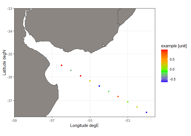
bounding box not fully supplied
plot_map(
    lon.min = -59,
    lat.max = -33,
    lats = seq(-35.5, -37.5, length.out = 10),
    lons = seq(-56.5, -52, length.out = 10),
    values = rnorm(10),
    value.name = "example [unit]"
)
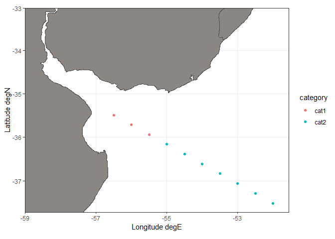
plot with categorical values
plot_map(
    lon.min = -59,
    lat.max = -33,
    lats = seq(-35.5, -37.5, length.out = 10),
    lons = seq(-56.5, -52, length.out = 10),
    values = c(rep("cat1", 3), rep("cat2", 7)),
    value.name = "category")
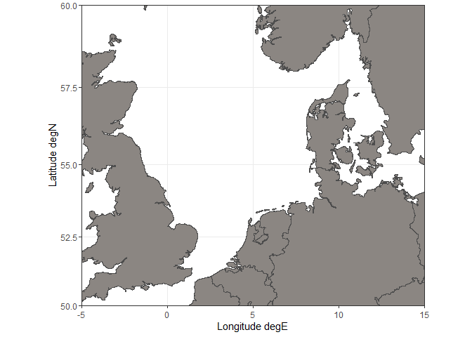
the function can also be used to make an empty
p1 <- plot_map(lon.min = -5, lon.max = 15, lat.min = 50, lat.max = 60)
p1
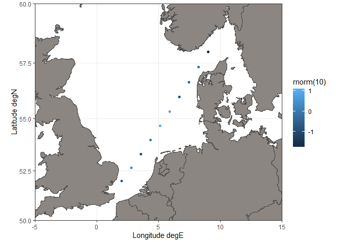
… which can then be filled with data
p1 + geom_point(aes(seq(2, 9, length.out = 10), seq(52, 58, length.out = 10), col = rnorm(10)))