Darshan01 / flows_pseudoaxions

Application of normalizing flows to BSM physics

• Current Bugs/Issues/"Features"
• Goals of Flows-Enriched Data Generation for High-Energy EXperiment (FEDHEX)
• Getting Started
  • Loading Training Data
  • Generating Training Data
  • Preprocessing Data
  • Running An Experiment
  • Generating New Data
  • Performing Analysis

Current Bugs/Issues/"Features"

• networks with multiple layers are not being saved or loaded correctly. They don't get evaluated correctly at the very least.
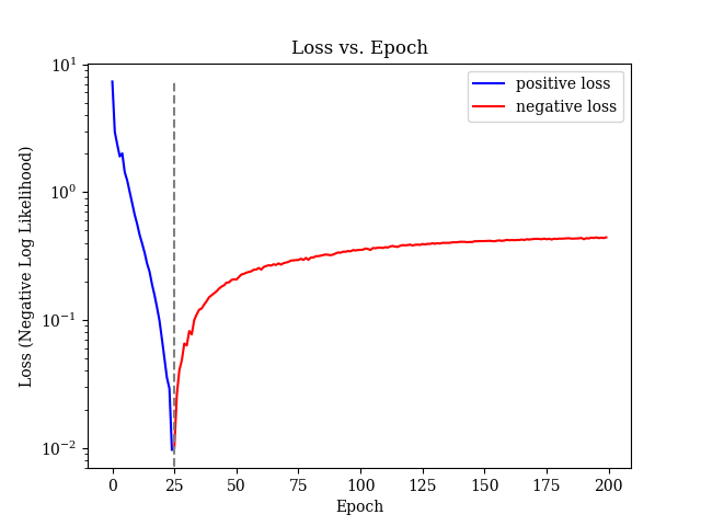
• The checkpointing callback does not save exactly at the epoch interval desired. I think this is likely a rounding issue as it looks to save based on the n-th batch, not the n-th epoch. So dividing total data size by batchsize produces yields an extra training step in the epoch to finish the last batch/cover the remainder. The math for the saving frequency for ckpt does not take this into account. Perhaps find a way to align checkpointing with epochs, though this is more an aesthetic/meta-accuracy thing than critical to the model's success.

Goals of Flows-Enriched Data Generation for High-Energy EXperiment (FEDHEX)

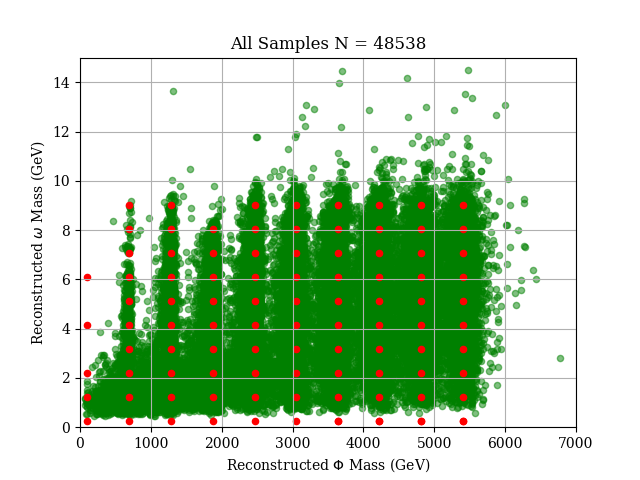
Given a sparse collection of event distributions in an N-dimensional parameter space, we want to interpolate between the given distributions to generate new distributions

For example, a hypothetical interaction between two particles, yielding a scalar $\Phi$ and pseudoaxion (pseudoscalar) $\omega$, can be modelled as such.

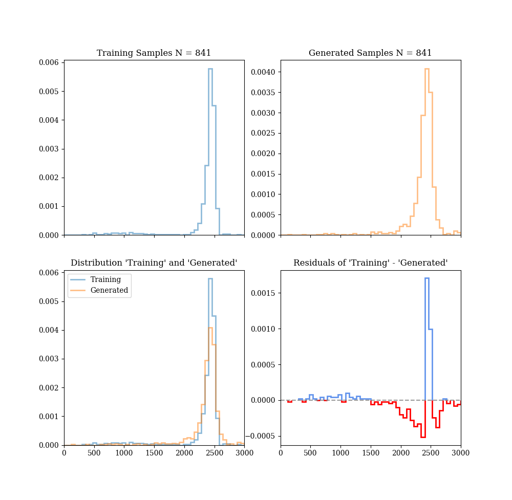
We wish to get the accuracy to within ~1% of MCMC-generated data.

Getting Started

Create a new environment using (ana/mini)conda package manager:

conda create -n flows3.10 --file requirements.txt

Check out some tutorial notebooks: tut_gaus.ipynb and tut_root.ipynb

Loading Training Data

Use the class RootLoader to load data from Numpy or .ROOT files.

import fedhex as fx
rl = fx.RootLoader(root_path)
samples, labels = rl.load()

Generating Training Data

Use the class Generator to generate data with a specific generation Strategy (for gaussian generators, these "Strategies" modify the covariance matrix for each generated gaussian)

from fedhex.pretrain.generation import DiagCov, RepeatStrategy
strat = RepeatStrategy(DiagCov(ndim=2, sigma=0.025))
generator = fx.GridGaussGenerator(cov_strat=strat, ndistx=5, ndisty=5)
samples, labels = generator.generate(nsamp=1000)

Preprocessing Data

Use any concrete subclass of DataManager subclass, e.g., RootLoader or GridGaussGenerator to pre-process the data using the preproc() function. The manager must have data loaded/generated to retrieve the network-ready data and conditional data:

data, cond = rl.preproc()

Running An Experiment

Use any concrete subclass of ModelManager, e.g., MADEManager or RNVPManager, to handle all of the model setup and running once all necessary parameters are provided.

Build a model with the given model parameters:

# Create MADEManager instance with all parameters needed to build model
mm = fx.MADEManager(nmade=nmade, ninputs=ninputs, ncinputs=ncinputs,
                    hidden_layers=hidden_layers, hidden_units=hidden_units,
                    lr_tuple=lr_tuple)

# Build model
mm.compile_model()

Make the callbacks for training:

# Make callbacks
from fedhex.train import Checkpointer, EpochLossHistory, SelectiveProgbarLogger

callbacks = []

save_freq = 50 * batch_size # Save model at checkpoints 50 epochs apart
callbacks.append(Checkpointer(filepath=flow_path, save_freq=save_freq))

callbacks.append(EpochLossHistory(loss_path=loss_path))

log_freq = 10 # Log training losses every 10 epochs
callbacks.append(SelectiveProgbarLogger(1, epoch_interval=log_freq, epoch_end=end_epoch))

Run a model with the given run parameters:

# Run training procedure
mm.train_model(data=data, cond=cond, batch_size=batch_size,
               starting_epoch=starting_epoch, end_epoch=end_epoch,
               path=path, callbacks=callbacks)

Generating New Data

Evaluate the model for specified conditional data:

# Setup sample generation for a known training label
ngen = 500
gen_labels_unique = [0.5, 0.5]
gen_labels = np.repeat([gen_labels_unique], ngen, axis=0)
gen_cond = rl.norm(gen_labels, is_cond=True)

# Generate data for the provided conditional data
gen_data = mm.eval_model(gen_cond)

# Denormalize data using known transformation parameters
gen_samples = rl.denorm(gen_data, is_cond=False)

Look how a model network performs:

Performing Analysis