This package provides the functionality of visualizing data on a standard brain surface. This package leverages brain visualization functionality available in the connectome workbench made available as part of the Human Connectome Project [1].
This package provides two visualization options:
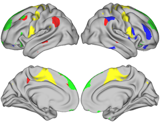
- Visualize selected regions of interest on the brain surface (see Fig 1)
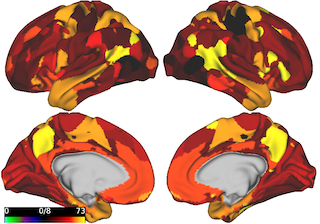
- Visualize a desired metric for each region in a brain parcellation (see Fig 2)
- Visualize a desired metric for each voxel in a brain parcellation
- Visualize a brain surface from data contained in a dscalar file
Figure 1: Visualizing 100 regions from ICA parcellation.
Figure 2: Visualizing multipole membership values for all regions in ICA parcellation.
Operating systems: Linux, OS X
Software:
- Workbench Command [2] that can be called using $wb_command
- For option 2 and 3:
- Julia v"1.0.x" with PyCall (v"1.91.4" tested)
- Python 3.x with nibabel (v"3.1.1" tested), numpy (v"1.18.2" tested)
- .scene: Used by the HCP Workbench program to generate scenes.
- .surf.gii: Contains a blank 3D brain model for visualization.
- CIFTY files: This file type usually contains a 2D matrix with the grayordinates as the row and another information as the column. [3]
- .dtseries.nii: Contains a 2D matrix mapping the grayordinates to their timeseries.
- .dlabel.nii: Contains a 2D matrix mapping the grayordinates to their respective labels. Another way to understand this is this file contains information about which region is the grayordinate in.
- .dscalar.nii: Contains a 2D matrix mapping the grayordinates to any scalar values.
1. Option 1
Description:
- Filter out the regions given in the input text file.
- Generate a new “.dlabel” file where the filtered regions are colored and the rest remain blank.
- Generate a visualization image of the selected regions.
How to run:
$chmod +x plotSelectedRegions.sh

$./plotSelectedRegions.sh input_file dlabel_file scene_file [output_file] [img_width] [img_height]
Input:
-
input_file : the text file (.txt) that contains the index of each region to be highlighted (option 1) or the value of each region (option 2).
Option 1: to highlight the regions of indices 2, 39, 45, the content of **input_file** shall consist of the following 3 lines: 2 39 45 Option 2: for a parcellation with n regions, the *input_file* shall consist of n rows only, in which row i represents the value of region i. -
dlabel_file : the dlabel file (.dlabel.nii) of the parcellation
-
scene_file : the scene file that specifies the background input files (.surf.gii for left and right hemispheres) and the view angle of the image
-
output_file (optional): the name (with path) of the output image. When this parameter is not provided, the output image will be saved as brain_image.png in ../
-
img_width (optional): the width of the output image in pixel. Default: 900
-
img_height (optional): the height of the output image in pixel. Default: 700
Output:
- Image file has the name specified by output_file if given or brain_image.png, otherwise
2. Option 2
Description:
- Used to map values to cortical surface regions (the outer part of the brain).
- Create a new “.dscalar” file that contains a mapping of the grayordinates (according to their regions) to the values specified in the input text file.
How to run
$julia plotRegionValues.jl val_file dlabel_file dscalar_file
Input:
- val_file : text file (.txt) that has on each row the pair of region index and value separated by ','
- dlabel_file : the standard dlabel file (.dlabel.nii) of the parcellation
- dscalar_file : the standard dscalar file (.dscalar.nii) of the parcellation
Output:
- Image file named brain_image.png in the current folder
3. Option 3
Description:
- Used to map values to subcortical voxels (the center part of the brain, connected to the spinal cord).
- Create a new “.dscalar” file that contains a mapping of the grayordinates (according to their voxels) to the values specified in the input text file.
How to run
$julia plotVoxelValues.jl val_file dlabel_file dscalar_file
Input:
- val_file : text file (.txt) that has on each row the pair of voxel index and value separated by ','
- dlabel_file : the standard dlabel file (.dlabel.nii) of the parcellation
- dscalar_file : the standard dscalar file (.dscalar.nii) of the parcellation
Output:
- Image file named brain_image.png in the current folder
4. Option 4
Description:
- Generate a visualization image from the provided “.scene” file and “.dscalar” file.
How to run
$./plotDscalar.sh input_file scene_file [output_file] [img_width] [img_height]
Input:
- input_file : input dscalar file (.dscalar.nii)
- scene_file : the scene file that specifies the background input files (.surf.gii for left and right hemispheres) and the view angle of the image
- output_file (optional): the name (with path) of the output image. When this parameter is not provided, the output image will be saved as brain_image.png in ../
- img_width (optional): the width of the output image in pixel. Default: 900
- img_height (optional): the height of the output image in pixel. Default: 700
[1] Human Connectome Project. https://www.humanconnectome.org
[2] Workbench. https://www.humanconnectome.org/software/workbench-command
[3] The minimal preprocessing pipelines for the Human Connectome Project https://www.sciencedirect.com/science/article/pii/S1053811913005053

