Catherine22 / Algorithms

Exercise for the Algorithms module by Princeton University.

Algorithms

Table of Contents

• Algorithms
  • Table of Contents
  • Equals
  • Dynamic Connectivity
    • Quick Find - An eager approach
    • Quick Union - A lazy approach
    • Improving quick find and quick union
    • Percolation
  • Stack
  • Queue
  • Sorting
    • Merge Sort
      • Merge sort with insertion sort
      • Merge sort with partially-ordered arrays
      • Bottom-up merge sort
    • Quick Sort
      • Quick sort with insertion sort
      • Estimating the partition
    • Heap Sort
    • Sorting in Practice
  • Priority Queues
    • Binary Heaps
    • Heap Sort
    • Symbol Tables
  • Balanced Search Trees
    • 2-3 Search Trees
    • Red-Black BSTs
    • 1d Range Search, One Dimensional Range Search
  • Hash Tables
  • References

Equals

In Java, all classes inherit a method equals(). For any references x, y and z, they must hit the following criteria:

1. Reflective: x.equals(x) is true.
2. Symmetric: x.equals(y) iff y.equals(x)
3. Transitive: If x.equals(y) and y.equals(z), then x.equals(z).
4. Non-null: x.equals(null) is false.

Best practices:

1. No need to use calculated fields that depend on other fields.
2. Compare fields most likely to differ first.
3. Make compareTo() consistent with equals(). I.e., x.equals(y) iff x.compareTo(y) == 0

x == y is equivalent to x.equals(y) when x and y are primitive types. Otherwise, user-defined types should be careful. Below is an example.

public final class Date implements Comparable<Date> {
    private final int day;
    private final int month;
    private final int year;

    public boolean equals(Object y) {
        if (y == this) {
            return true;
        }

        if (y == null) {
            return false;
        }

        // Object must be in the same class (religion: getClass() vs instanceof())
        if (y.getClass() != this.getClass()) {
            return false;
        }

        // Case is guaranteed to succeed
        Date that = (Date) y;

        // Check if all the significant fields are all the same
        if (this.day != that.day) {
            return false;
        }

        if (this.month != that.month) {
            return false;
        }

        if (this.year != that.year) {
            return false;
        }

        return true;
    }
}

If x and y are arrays, the above rules should apply to each entry.

Dynamic Connectivity

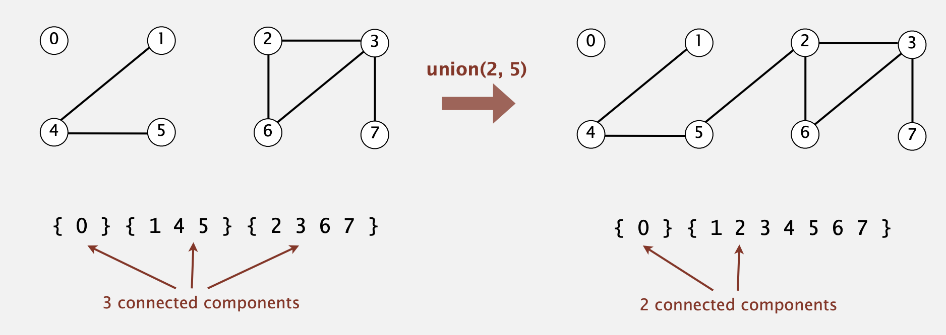
Given a set of N objects. A union-find class includes:

• UF(int N): The constructor of the UF class that initialises a union-find data structure with N objects.
• void union(a, b): A union command connects two objects.
• boolean find/connect(a, b): Are a and b in the same component?

Quick Find - An eager approach

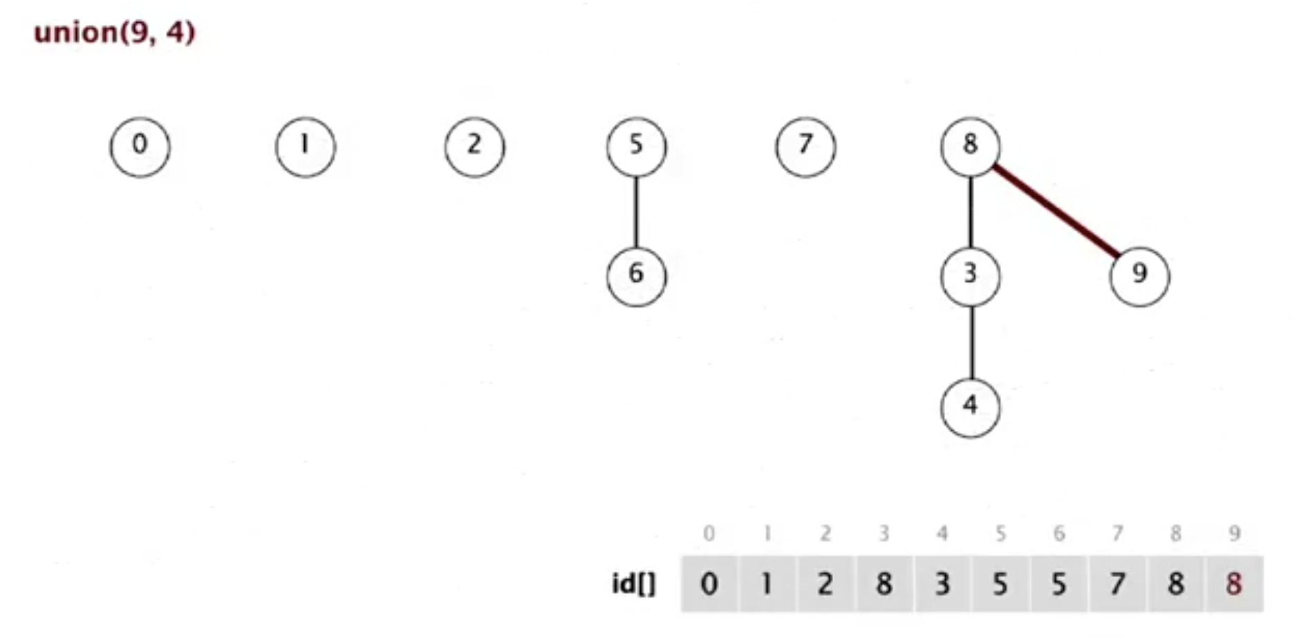
In quick union, we need an array to keep nodes' locations. For each node i, the array id[i] keeps where the node i points to. When node p unions to q, we must loop the array and replace all the values that equal to id[p] with id[q] .

Example 1

[0, 1, 2, 3, 4, 5, 6, 7, 8, 9] -> union(4, 3)
[0, 1, 2, 3, 3, 5, 6, 7, 8, 9] -> union(3, 8)
[0, 1, 2, 8, 8, 5, 6, 7, 8, 9] -> union(6, 5)
[0, 1, 2, 8, 8, 5, 5, 7, 8, 9] -> union(9, 4)
[0, 1, 2, 8, 8, 5, 5, 7, 8, 8] -> union(2, 1)
[0, 1, 1, 8, 8, 5, 5, 7, 8, 8] -> union(5, 0)
[0, 1, 1, 8, 8, 0, 0, 7, 8, 8] -> union(7, 2)
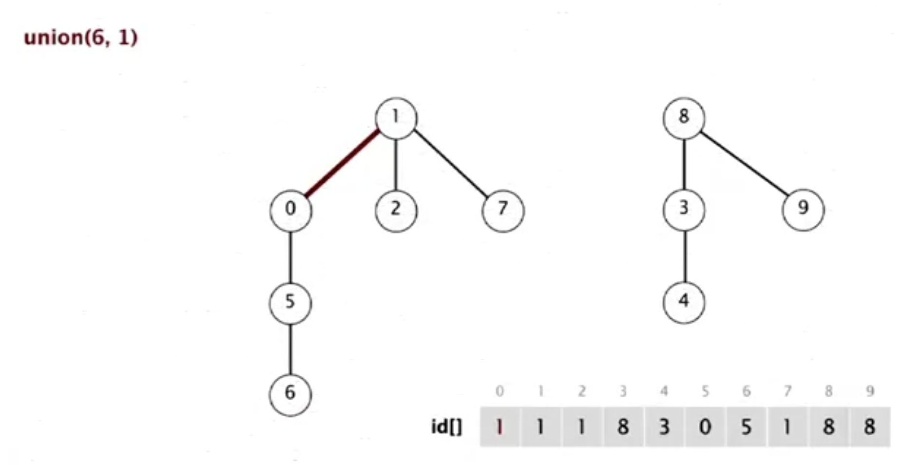
[0, 1, 1, 8, 8, 0, 0, 1, 8, 8] -> union(6, 1)
[1, 1, 1, 8, 8, 1, 1, 1, 8, 8] -> connected(0, 2)
true // array[0] == array[2]

Quick Union - A lazy approach

Quick-find is too slow for huge problems. An alternative is called quick union. In quick union, we need an array to keep nodes' locations. For each node i, the array id[i] keeps where the node i points to. E.g., id[0] = 0 means the node 0 has no parents. id[3] = 9 means the node 3 is pointing to the node 9. When node p points to node q, the root of p points to the root of q. E.g.,

   i    0  1  2  3  4  5  6  7  8  9
-------------------------------------
id[i]   0  9  6  5  4  2  6  1  0  5

The roots of 3 and 7 are both 6.

Improving quick find and quick union

Algorithm	Initialise	Union	Find
Quick Find	N	N	1
Quick Union	N	N	N
Weighted QU	N	log N	log N

If the tree becomes flatter, the cost of find in the quick union will be less. Weighted quick union is an improvement of the quick union. Instead of joining the root of p to the root of q, it compares the size of trees where p and q are and merge the root with a smaller tree to the other root.

Percolation

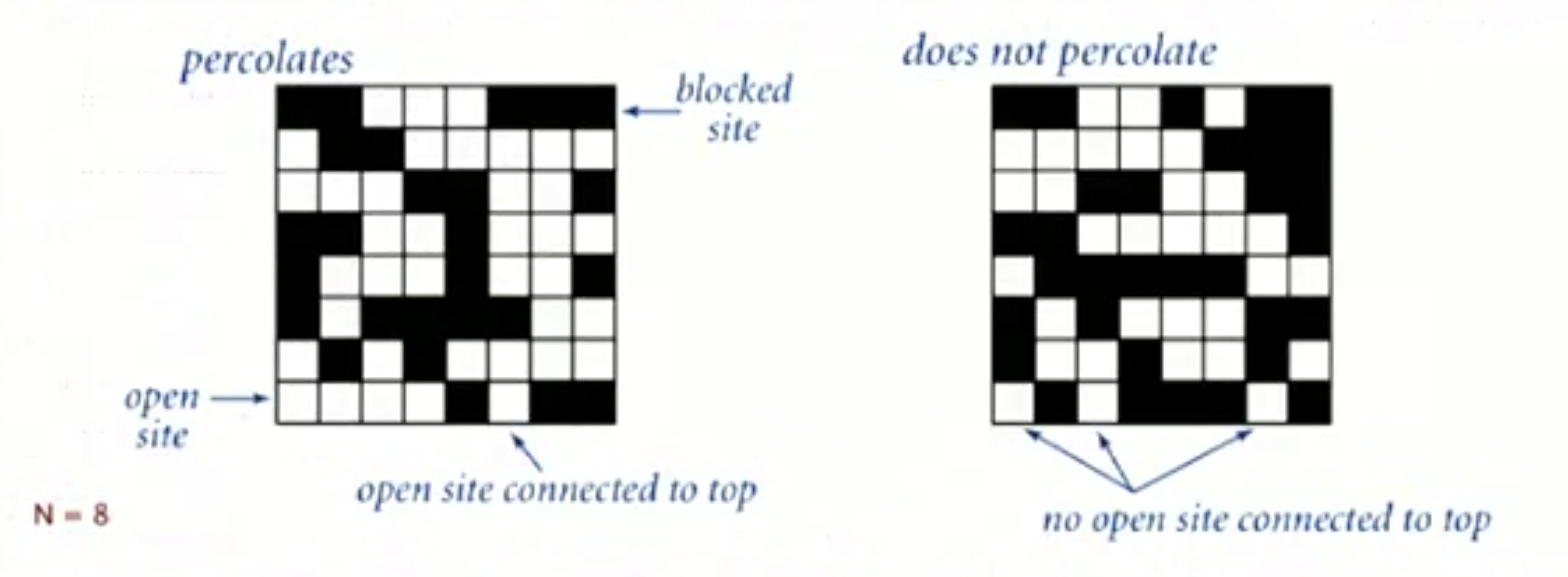
The Union-Find is a model for many physical systems, specifically, systems percolates iff top and bottom are connected by open sites.

programming assignment: percolation

Stack

Stacks

Queue

Queues

Sorting

Merge Sort

MergeSort.java

Merge sort is com used as a primary sorting method in programming languages.

Merge sort with insertion sort

Merge sort is too expensive for tiny arrays and has too much overhead for tiny subarrays. An improvement of merge sort is to cut off and use insertion sort to sort for tiny subarrays.

For example, in MergeSort.java, we have the following code:

private void sort(Comparable<T> a[], Comparable<T> aux[], int lo, int hi) {
    if (hi <= lo) {
        return;
    }
    int mid = (lo + hi) / 2;
    sort(a, aux, lo, mid);
    sort(a, aux, mid + 1, hi);
    merge(a, aux, lo, mid, hi);
}

With insertion sort, it becomes:

private final static int CUTOFF = 7;
private void sort(Comparable<T> a[], Comparable<T> aux[], int lo, int hi) {
    if (hi <= lo + CUTOFF - 1) {
        InsertionSort.sort(a, lo, hi);
        return;
    }
    int mid = (lo + hi) / 2;
    sort(a, aux, lo, mid);
    sort(a, aux, mid + 1, hi);
    merge(a, aux, lo, mid, hi);
}

Merge sort with partially-ordered arrays

Another approach to improve merge sort is to stop sorting when subarrays are partially sorted.

private void sort(Comparable<T> a[], Comparable<T> aux[], int lo, int hi) {
    if (hi <= lo) {
        return;
    }
    int mid = (lo + hi) / 2;
    sort(a, aux, lo, mid);
    sort(a, aux, mid + 1, hi);
    if (a[mid].compareTo((T) a[mid + 1]) <= 0) {
        return;
    }
    merge(a, aux, lo, mid, hi);
}

Bottom-up merge sort

An implementation of the merge sort without recursion is called the bottom-up merge sort. It works as follows:

[4, 2, 6, 8, 1, 5, 3, 9]
 ----
[2, 4, 6, 8, 1, 5, 3, 9]
       ----
[2, 4, 6, 8, 1, 5, 3, 9]
             ----
[2, 4, 6, 8, 1, 5, 3, 9]
                   ----
[2, 4, 6, 8, 1, 5, 3, 9]
 ----------
[2, 4, 6, 8, 1, 5, 3, 9]
             ----------
[2, 4, 6, 8, 1, 3, 5, 9]
 ----------------------
[1, 2, 3, 4, 5, 6, 8, 9]

Check out MergeSortBottomUp.java to see if it works.

Quick Sort

QuickSort.java

In quick sort, we have a function called partition, where we have two pointers, i and j, and lo refers to the lowest element. We start from i = lo + 1, ensuring that all elements between i and j are lesser than a[lo]. j, on the other hand, is initially equal tohi (the highest element). We ensure the subarray ranged from j to hi is greater than a[lo]. We stop the above checking while j is less than or equal to i. Then we exchange a[lo] and a[j].

Below shows how partition works:

before
[x|                       ]
[l]                     [j]

during
[x| <=x  |       |   >=x  ]
        [i]     [j]       ]

after
[    <=x    |x|    >=x    ]
[l]         [j]         [h]

It is noticeable that we must shuffle the array before actual partition and sorting to have a probabilistic guarantee against the worst case.

Quick sort with insertion sort

The way we add insertion sort to quicksort is the same as we do in merge sort. This time, the CUTOFF is 10.

private final static int CUTOFF = 10;
private void sort(T[] a, int lo, int hi) {
    if (hi <= lo + CUTOFF - 1) {
        InsertionSort.sort(a, lo, hi);
        return;
    }

    int j = partition(a, lo, hi); // j is the correct position, no need to check j again.
    sort(a, lo, j - 1);
    sort(a, j + 1, hi);
}

Estimating the partition

Another improvement of quicksort is to estimate the partitioning element being near the middle rather than arbitrarily use the first element, which, on average, will be at the middle. The method is to sample the items and take the median of the sample. This improvement is not usually worth the cost of enlarged samples. Three times can slightly reduce the number of comparisons and increase the number of exchanges paradoxically.

private void sort(T[] a, int lo, int hi) {
    if (hi <= lo) {
        return;
    }

    int m = medianOf3(a, lo, (lo + hi) / 2, hi);
    exch(a, lo, m);
    int j = partition(a, lo, hi); // j is the correct position, no need to check j again.
    sort(a, lo, j - 1);
    sort(a, j + 1, hi);
}

Heap Sort

Check out Heap Sort.

Sorting in Practice

1. Given an array of N items, find a kth smallest item.

In this example, we simplify the partition method from quicksort by using one single pointer as follows:

before
[                         ]
[l]                     [h]

after
[    <=j    |j|    >=j    ]
[l]         [k]         [h]

Check out Selection.java

2. Huge numbers of duplicate keys

The solution is to adopt 3-way partitioning. It is a little bit complicated than a standard partitioning method in quicksort.

before
[v|                     ]
[l]                    [h]
duration
[ < v | = v |     | > v ]
      [lt]  [i]   [gt]
after
[  < v  |  = v  |  > v  ]
[l]     [lt] [gt]     [h]

Check out DuplicateKeys.java

Priority Queues

Binary Heaps

Proposition

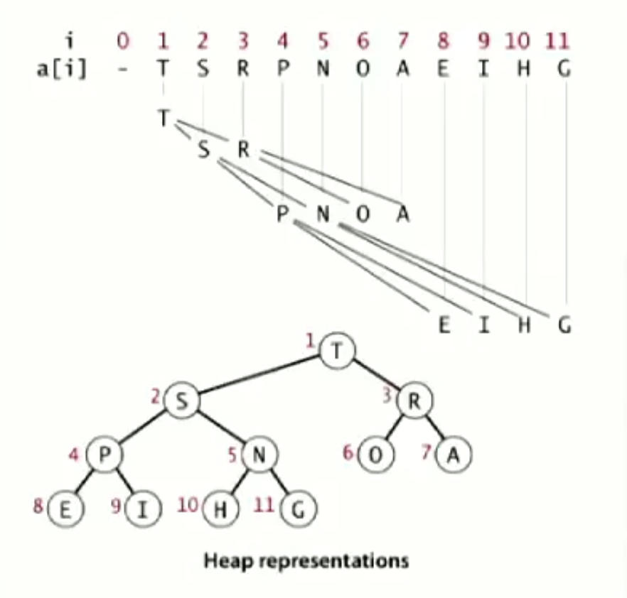
• Largest key is a1, which is root of binary tree.
• Parent of node at k is at k/2.
• Children of node at k are at 2k and 2k+1.

Promotion in a heap

Scenario: Child's key becomes larger key than its parent's key.

To eliminate the violation, we have to exchange the key in the child with the key in the parent. After that exchange, check if the parent's key is larger than its parent. Finally, we repeat the exchange up to the root.

Demotion in a heap

Scenario: Parent's key becomes smaller than one (or both) of its children's.

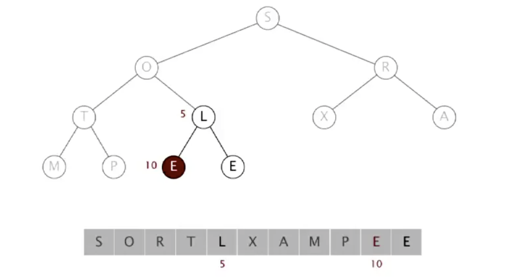
To eliminate the violation, we have to exchange the parent's key with the child's key. After that exchange, check if the child's key is smaller than its children. If so, exchange the child's key and its' largest child's. Repeat the exchange until the heap order resorted.

Check out BinaryHeap.java.

Heap Sort

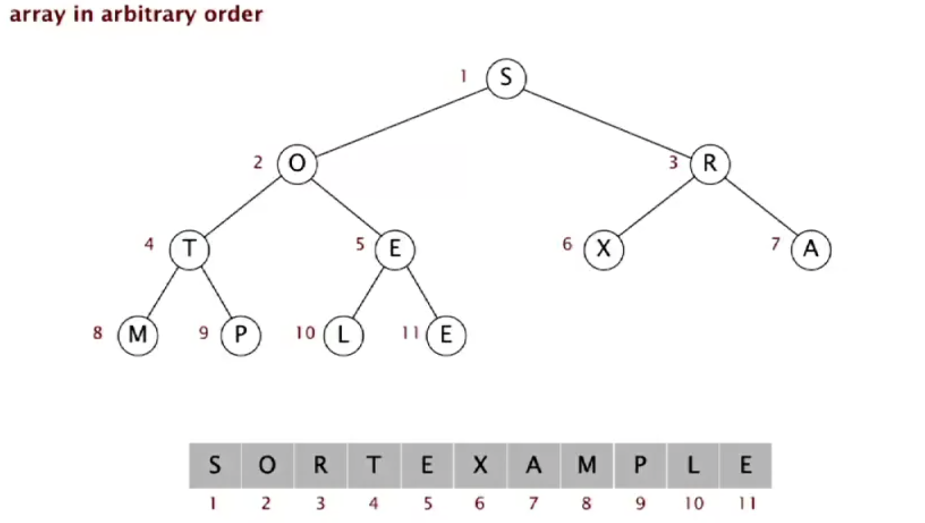
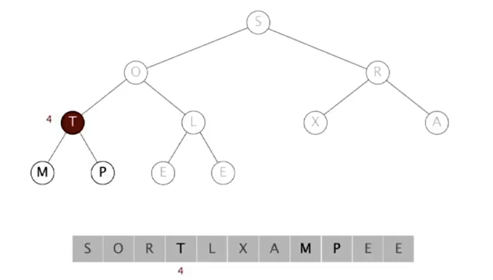
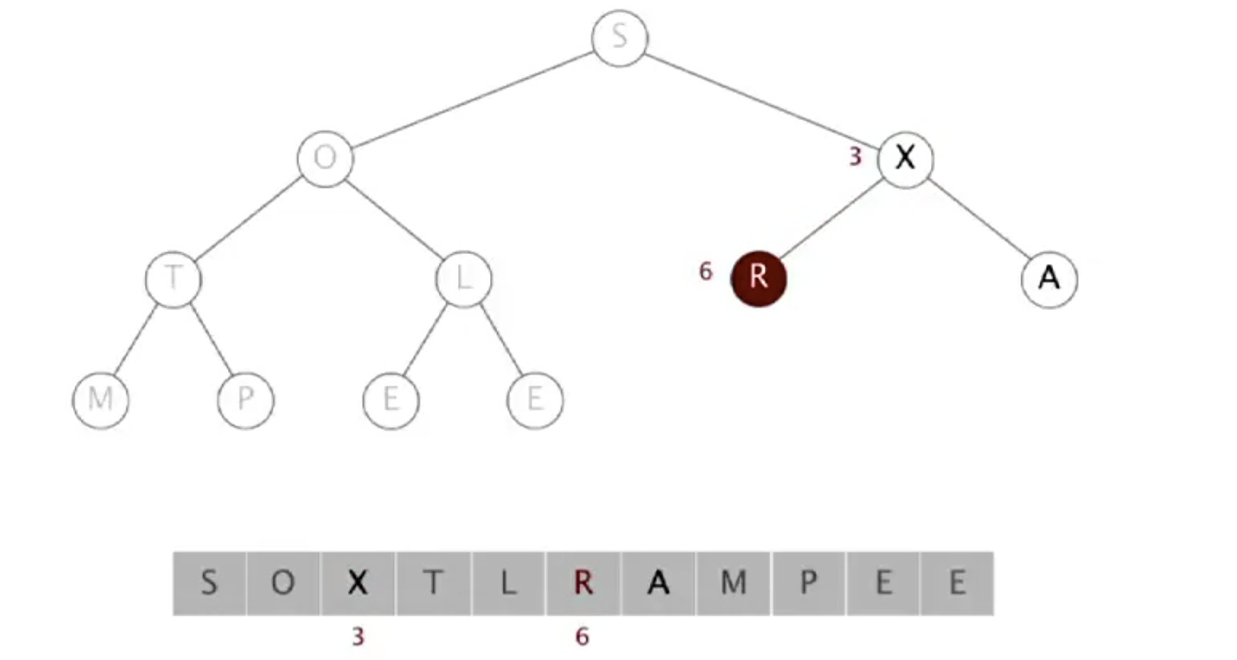
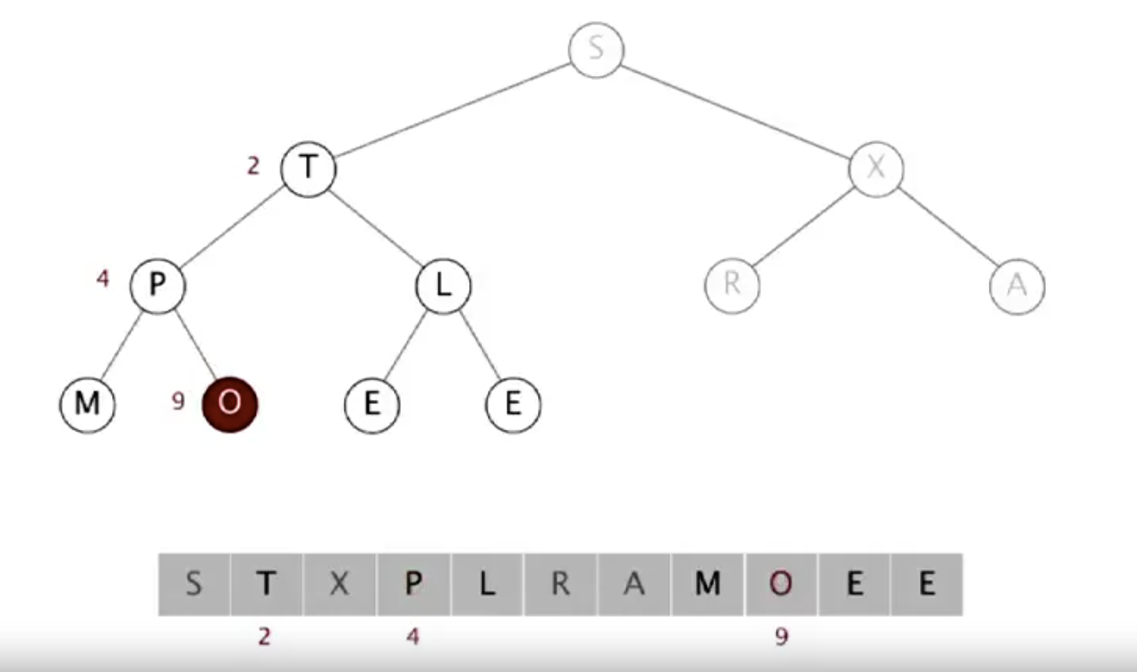
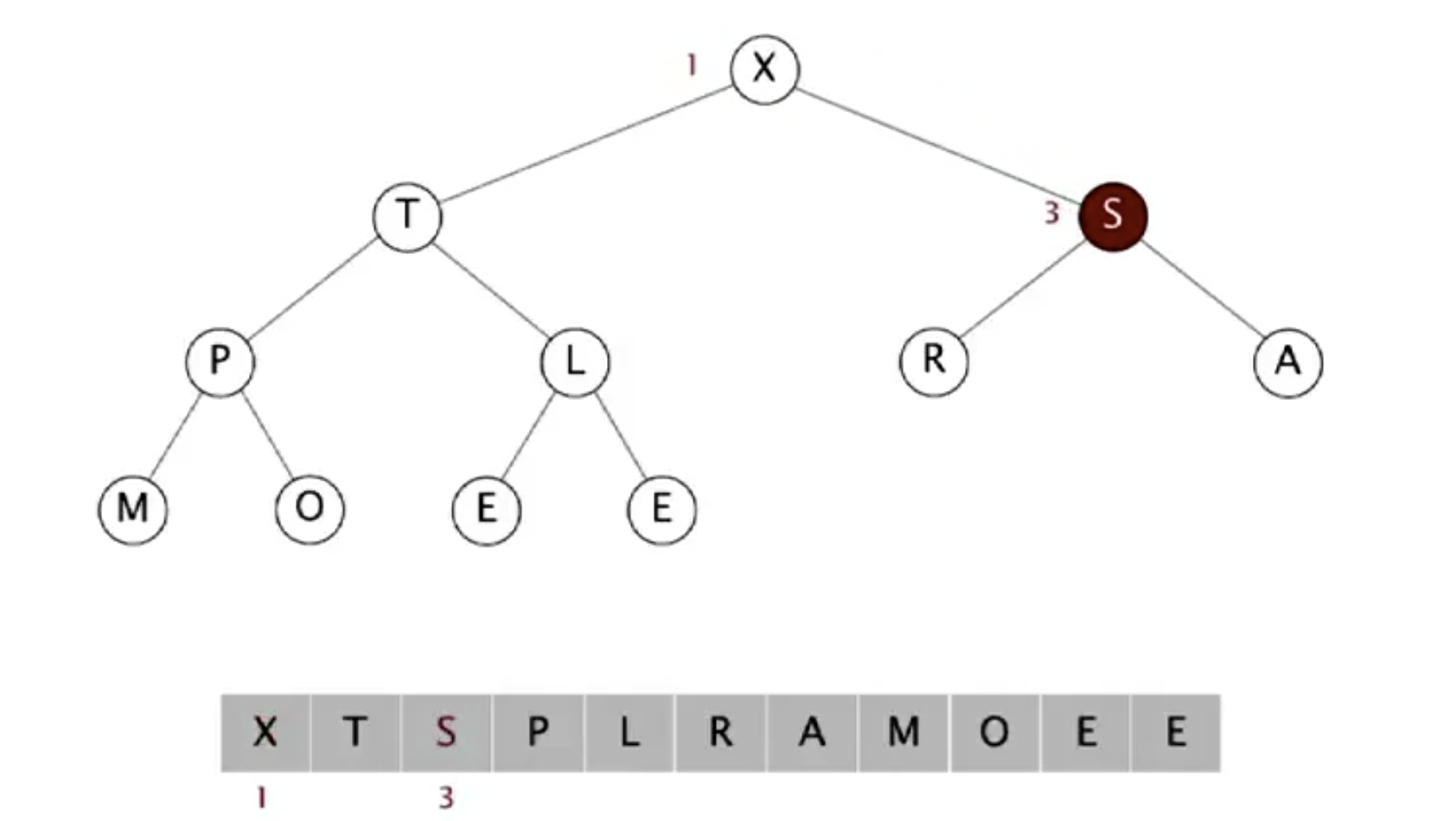
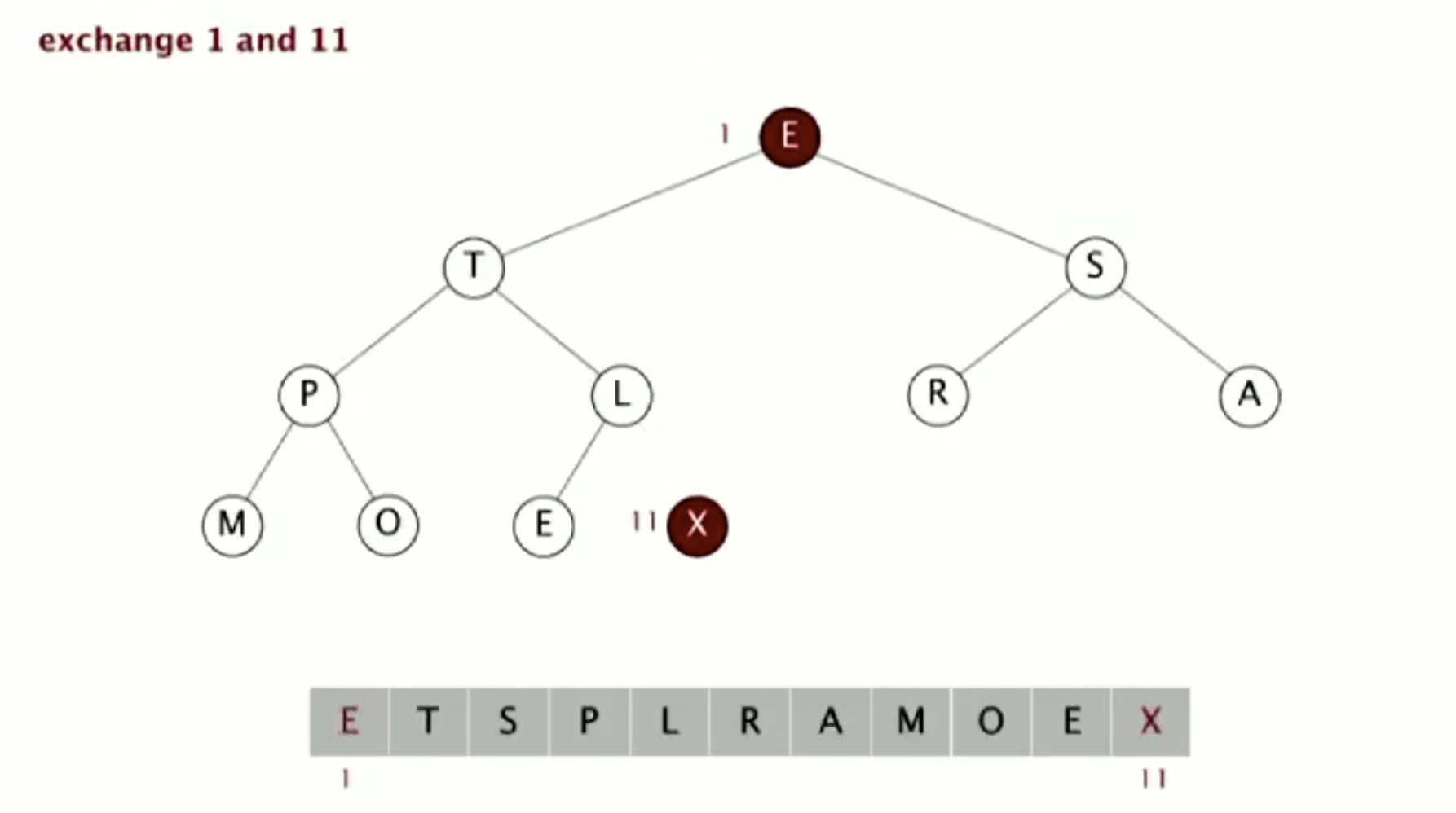
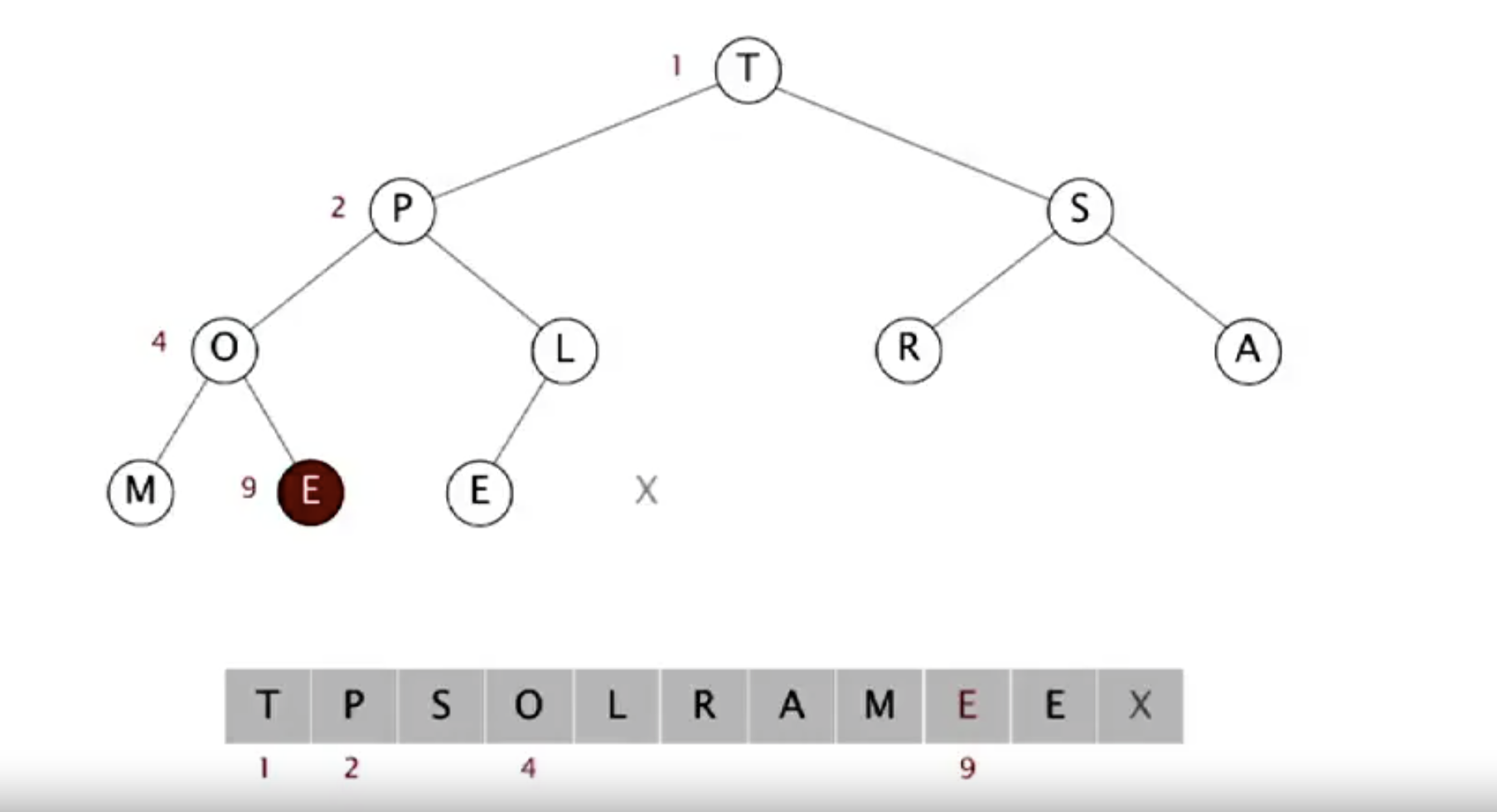
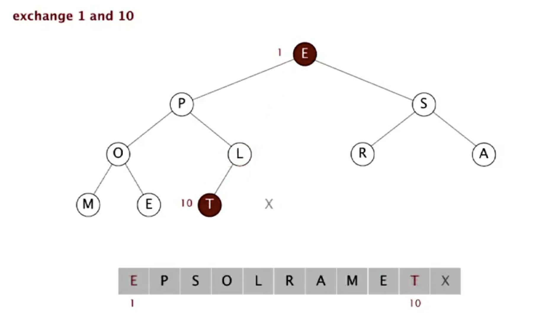
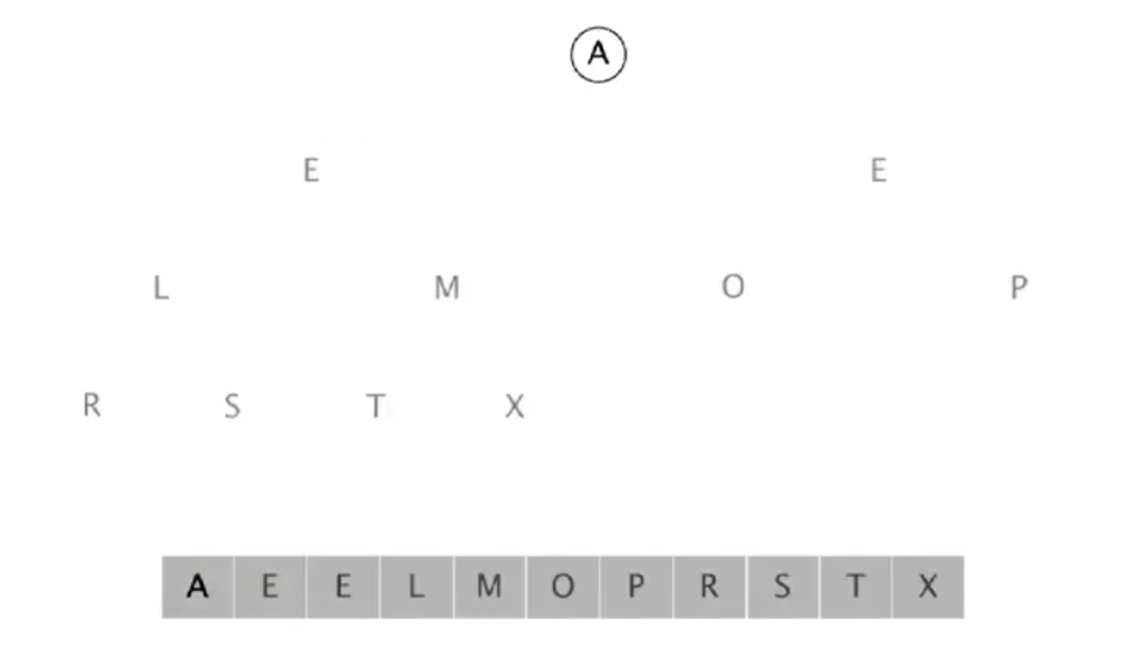
Implementation of the binary heap is heap sort. In heap sort, we exchange the root (the max value) with the last node, remove the old root and sink the new root until finding the second largest value. Then we repeat those three steps until all the nodes have checked. Detailed steps are shown below.

	complexity
Worst case time	O(N log(N))
Best case time	O(N)
Average case time	O(N log(N))
Space	O(1)

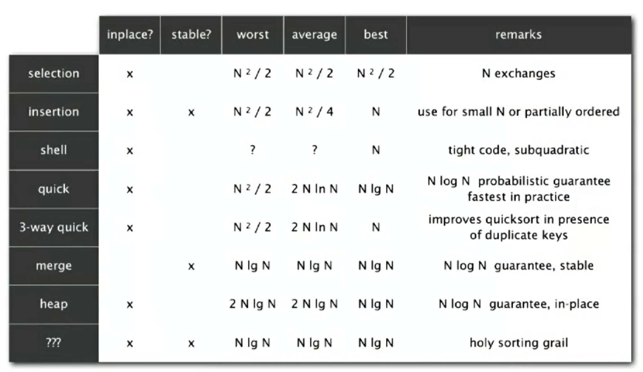
Although somewhat slower in practice on most machines than a well-implemented quicksort, it has the advantage of a more favorable worst-case O(n log n) runtime. Heapsort is an in-place algorithm, but it is not a stable sort [1].

Exchange the max value with the node at the end. Then we fix the max value.

Sink the new root.

Repeat the above two steps, exchanging the max value with the node at the end. This time, we fix the max value on the left of the previous fixed node.

Finish the loop when all the nodes have been fixed.

Check out HeapSort.java.

Symbol Tables

A symbol table is a key-value pair abstraction. For example, DNS lookup uses URLs as keys and IP addresses as values. In Java, a symbol table implements associative array abstraction, which associates one value with each key.

Balanced Search Trees

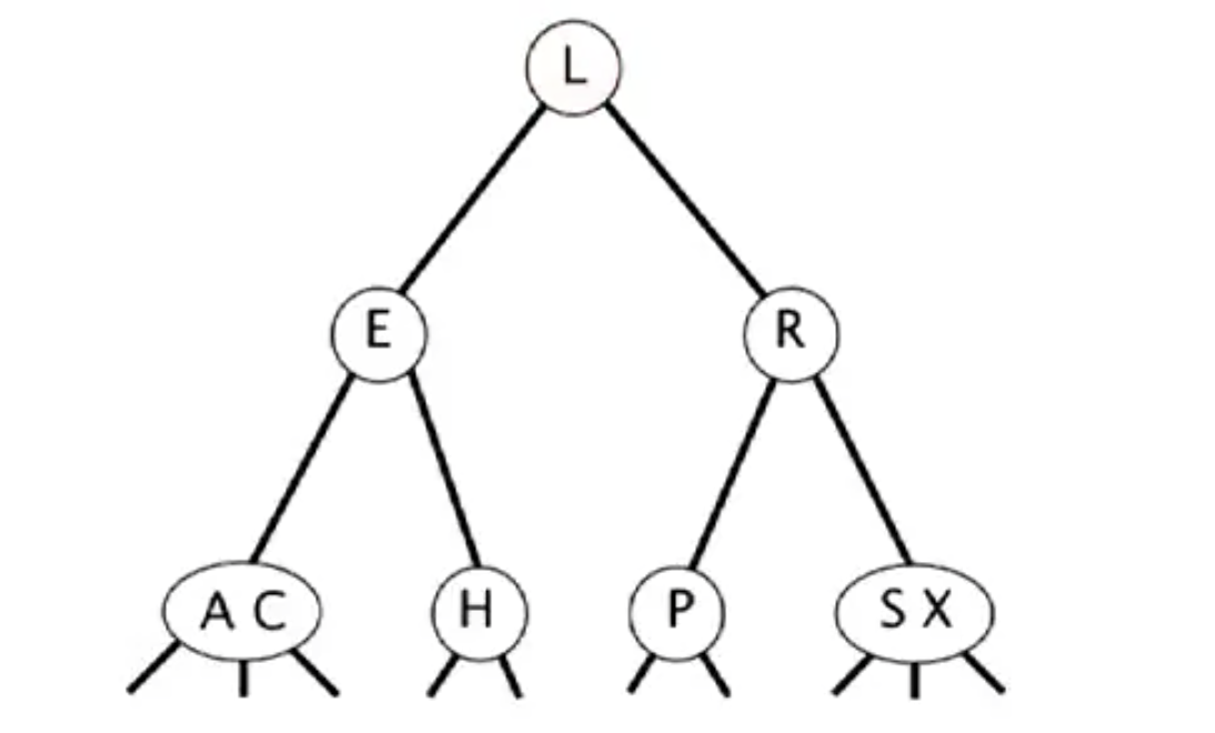
2-3 Search Trees

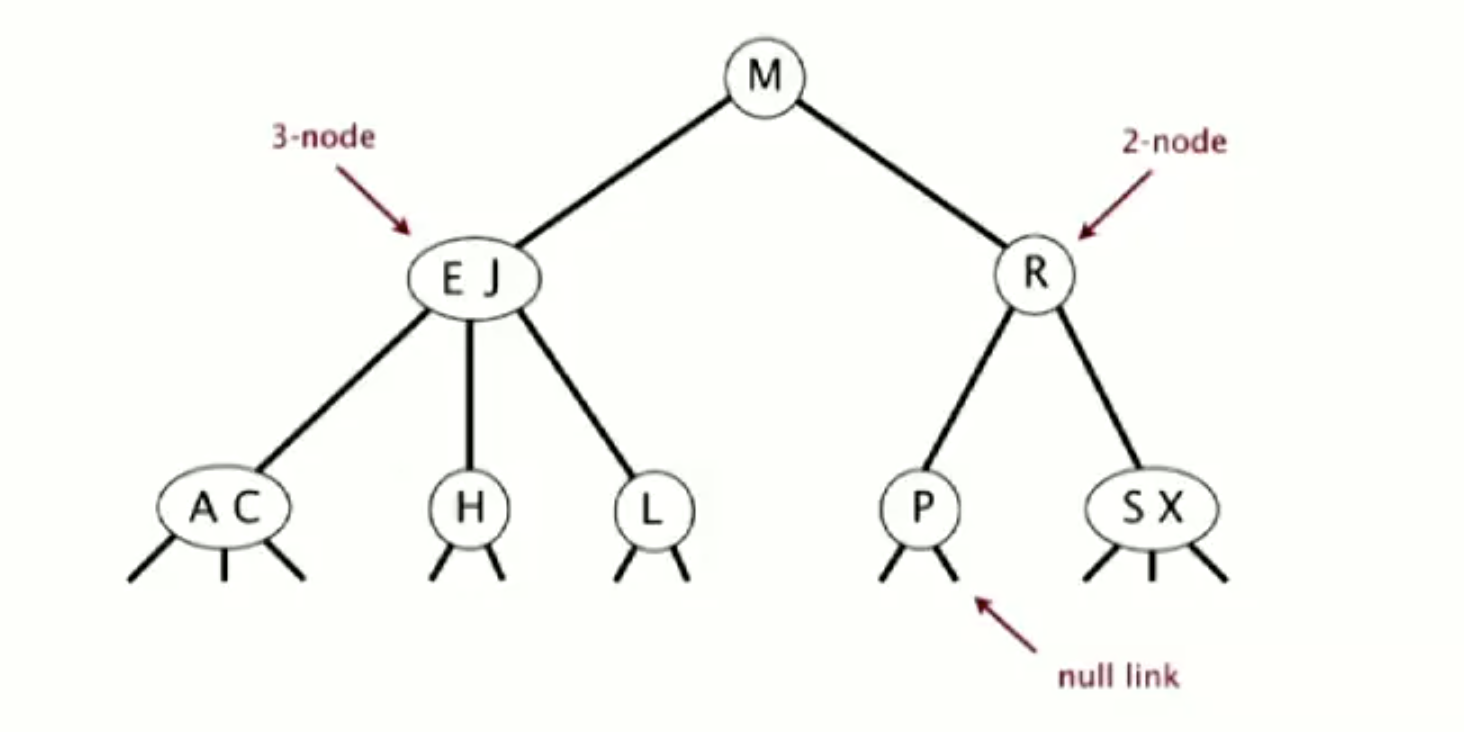
A 2-3 tree allows 1 or 2 keys per node:

• 2-node: 1 key, 2 children
• 3-node: 2 keys, 3 children

When a 2-3 tree is perfectly balanced, it suggests that every path from the root to a null link has the same length.

As the properties of the 2-3 tree, we know that a node can have at most three children, filling with two keys for each. Since the 2-3 tree is sorted, a right child must be larger than its siblings on the left, so do the keys. A one-key node is greater than its left child but smaller than its right child. A two-key node works as follows: left child < left key < median child < right key < right child.

Search

A search function starts from the root and goes down, comparing the target with the current node.

Insert

Traversing from the root as the search function does and reach to the bottom of the tree. There are two possible scenarios to handle when adding a key to an existed node as follows:

1. Adding a key to a one-key node: Replacing that 2-node with 3-node, placing the key on the left if it is smaller than another key and vice versa.
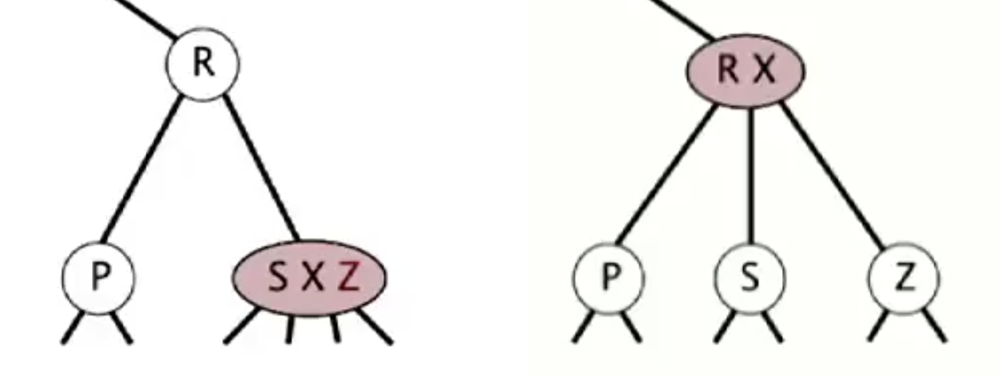
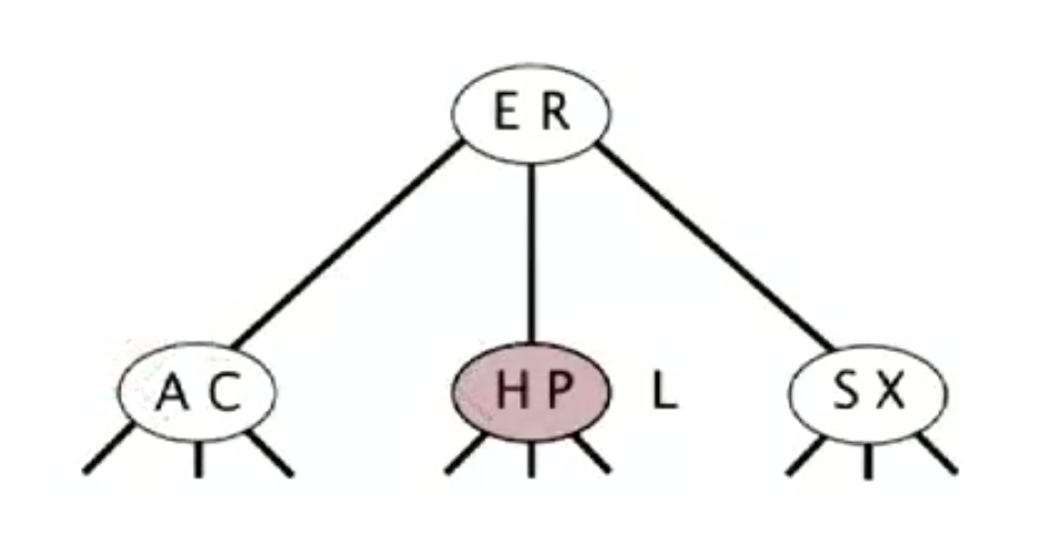
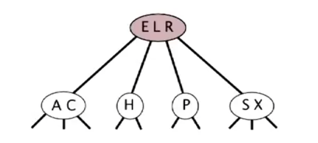
2. Adding a key to a two-key node:: We first have to temporarily merge that key to a 3-node even though it breaches the 2-3 tree policy. Then we pass the middle key in that 4-node up to its parent. Finally, we make sure the parent and its children comply with the rules of the 2-3 tree. Here are some examples:

E.g. Inserting Z

E.g. Inserting L

Red-Black BSTs

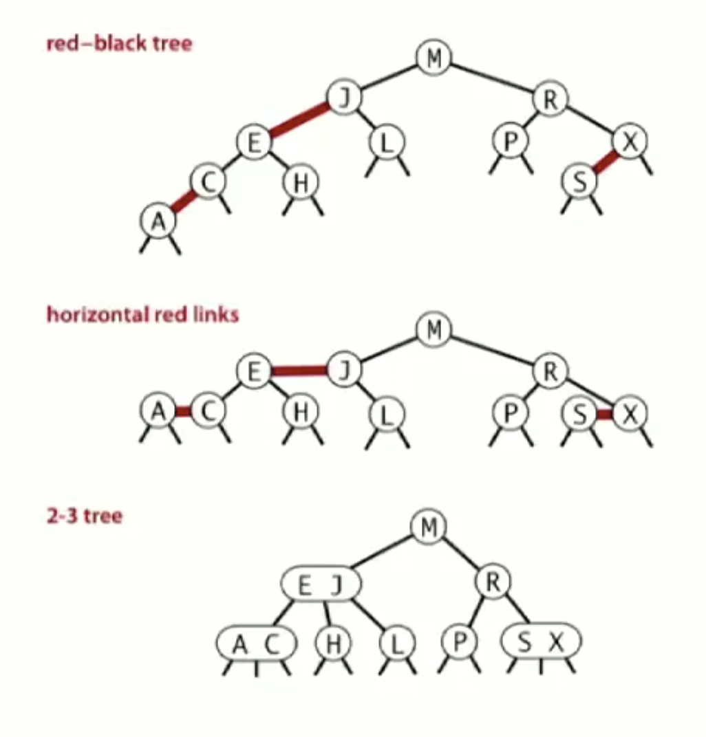
A red-black binary search tree is a simple way to implement the 2-3 three, which represents a 2-3 tree as a BST. The illustrations below are left-leaning red-black BSTs.

• If the link between two nodes is red, they are representations of a two-key node in the 2-3 tree.

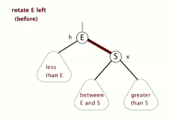
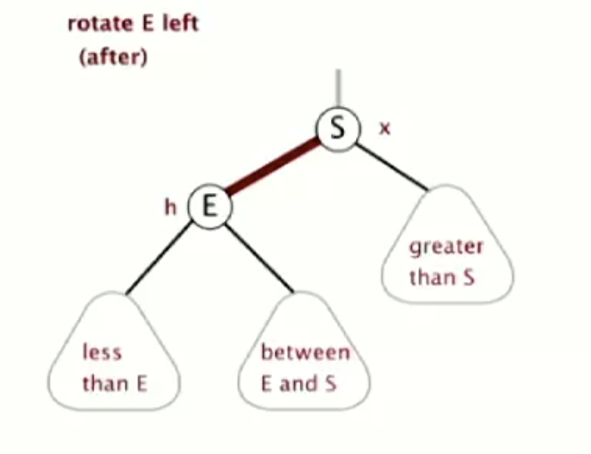
Rotate left

Orient a (temporarily) right-leaning red link to lean left.

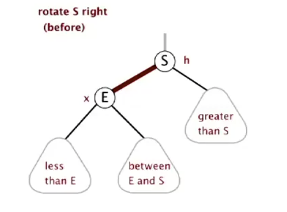
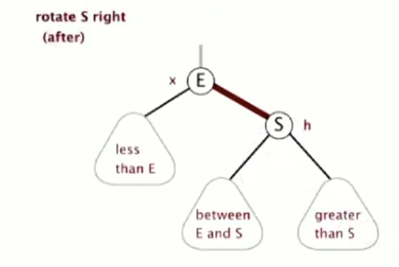
Rotate right

Orient a left-leaning red link to (temporarily) lean right.

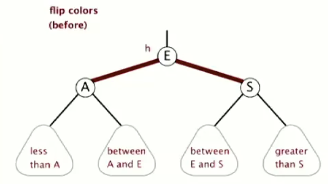
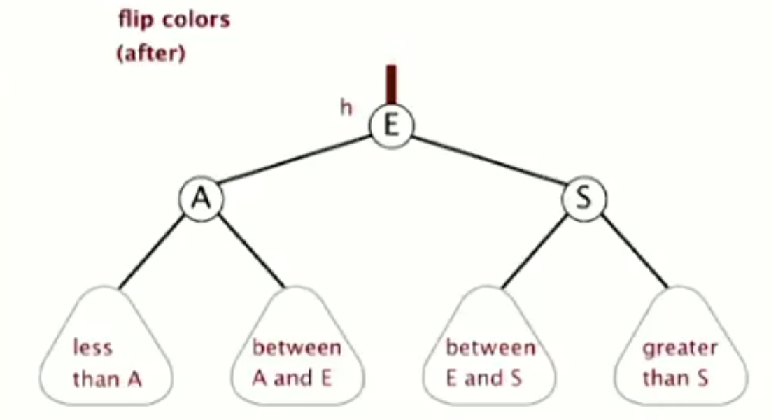
Flip colours

When we have a temporary 4-node as a 2-3 tree, we need to flip colours.

LLRBTree.java shows how to implement insertion for the LLRB tree.

1d Range Search, One Dimensional Range Search

Hash Tables

Below are the criteria of hashing:

• A hash function
• Equality test: A method for checking whether two keys are equal.
• Collision resolution: A collision is when two keys hash to the same index. We need an algorithm to handle collisions.

Therefore, a hash is a classic time-space tradeoff. Without space limitation, a trivial hash function uses a key as an index. Without time limitation, a trivial collision resolution uses sequential search. In the real world, the ideological goal is to ensure the hash function is efficiently computable and every table index equally likely for each key.

References

• Algorithms, Part 1
• Algorithms, Part 2
• Google Java Style Guide