Networkqit: spectral entropies of complex networks

An information theoretic approach inspired by quantum statistical mechanics was recently proposed as a means to optimize network models and to assess their likelihood against synthetic and real-world networks. Importantly, this method does not rely on specific topological features or network descriptors, but leverages entropy-based measures of network distance. Entertaining the analogy with thermodynamics, networkqit provides a computational tool for the estimate of spectral entropy and fitting of model parameters. These results enable the practical application of this novel and powerful framework to network model inference.

Documentation

The full documentation for this package under development and is currently being written, its current version is available at:

https://networkqit.github.io/

Installation

To use the networkqit package we suggest to use virtualenv. The networkqit package is pure Python, so it should work on Linux, Mac OSX and Windows. Here we report instructions for usage in a standard Ubuntu linux installation.

How to install on Linux

Open a terminal, install pip and virtualenv and clone this repository

sudo apt-get install python3-pip
sudo pip3 install virtualenv
virtualenv workspace
cd workspace
git clone https://github.com/carlonicolini/networkqit

You cloned the repository. Now start the virtualenv session.

source bin/activate

If you are inside the virtualenv session, check that the Python version you are using is the one provided by virtualenv.

which python3

Now install the networkqit package within the virtualenv environment.

cd networkqit
python3 setup.py sdist

Now install the created Python package, that should come with all its dependencies matplotlib, numpy, networkx, pandas, numdifftools, bctpy

cd ..
pip3 install networkqit/dist/networkqit-0.1.tar.gz

Getting started

Here we discuss how to use networkqit.

Computing the spectral entropy of a network

Let us start by studying the spectral entropy of the density matrix of the famous karate club graph. This example shows how to generate the spectral entropy plots shown in our main paper.

import networkx as nx
G = nx.karate_club_graph()
A = nx.to_numpy_array(G)
import networkqit as nq
import numpy as np
import matplotlib.pyplot as plt
plt.style.use('ggplot')
beta_range = np.logspace(-3,3,200)
Sbeta = nq.batch_compute_vonneumann_entropy(L=nq.graph_Laplacian(A),beta_range=beta_range)
plt.semilogx(beta_range, Sbeta)
plt.xlabel('$\\beta$')
plt.ylabel('$S$')
plt.title('Unnormalized spectral entropy')
plt.show()

The spectral entropy is always in the range [0, log(N)], so if we simply divide by log N where $N$ is the number of nodes, we renormalize it in the [0,1] range.

Generative network models

networkqit features a large number of network models, mainly those obtained from within the Maximum Entropy framework. You can create a number of models and call methods on them by a consistent nomenclature: Here we create an instance of the Undirected Binary Configuration model (UBCM), and sample 10 random networks from this ensemble, based on the fitness parameters x_i created at random in the [0,1] domain.

import networkqit as nq
N=10
model = nq.UBCM(N=10)
xi = np.random.random([N,])
adj_graphs = model.sample_adjacency(xi, batch_size=5)
print(adj_graphs.shape)

The call returns a [5,N,N] numpy array, where the last two dimensions embed with the adjacency matrix of the 5 random graphs. The method sample_adjacency is available for every generative model implemented in networkqit and is at the base of the maximize and sample approach used for the optimization of the spectral entropy.

Classical optimization of spectral entropies

Networkqit can also work with network model fitting. The utilities to define model optimization are defined in the algorithms package, and here we describe how to run model optimization in the non-sparse limit (the one discussed in the PRE paper).

The following lines describe an example of optimization of the expected Laplacian model. We first create the object ErdosRenyi that describes the expected Laplacian, adjacency and Laplacian gradient with respect to the only continuous parameters $p$.

import networkx as nx
import networkqit as nq
import numpy as np
G = nx.karate_club_graph()
A = nx.to_numpy_array(G)
L = nq.graph_Laplacian(A)
beta_range = np.logspace(-3,3,20)
ermodel = nq.ErdosRenyi(N=len(A))

We can call the ermodel as if it is a simple function:

print(ermodel([0.5]))

This returns the expected adjacency matrix, a 34x34 matrix with 0.5 off diagonal and 0 on diagonal. The ermodel also allows to call methods like the expected Laplacian or the expected Laplacian gradients:

print(ermodel.expected_Laplacian_grad([0.5]))

Otherwise we can sample 10 independent networks from the Erdos-Renyi model, with the method sample_adjacency:

print(ermodel.sample_adjacency([0.5]), batch_size=10)

Once the ermodel object is defined, we can optimize its parameters in the spectral entropies framework with the help of the class ContinuousOptimizer. We initialize the observed adjacency matrix as A and the initial solution x0=np.array([0.2]). It is important to define x0 as a numpy array. Finally the beta_range is a numpy array with the range of beta over which to optimize the model.

solver = nq.ContinuousOptimizer(A=A, x0=np.array([0.2]), beta_range=beta_range)
solver.setup(ermodel, ermodel.expected_Laplacian_grad, step_callback=None)
sol = solver.run()
print(sol)

Stochastic optimization of spectral entropy

Most of the models do not allow an analytical treatment of their spectral likelihood. This involves knowing exact analytical formulations of the Laplacian eigenvalues spectral density and this is still an unsolved problem for most of the useful network models. To perform spectral likelihood optimization we can do stochastic optimization and find the parameters of the empirical graph such that the expected relative entropy averaged over the model ensemble is minimized. Doing this in networkqit is simple, as the library relies on the autograd package for the automatic calculation of complicated gradients of stochastic functions.

With the optimization method Adam which is borrowed from machine learning, we can optimize the expected relative entropy of the Erdos-Renyi model with respect to our model karate-club network,represented by A and see the effects of changing the inverse temperature parameter beta on the optimization process.

At every iteration, a batch_size number of random networks are sampled from the model, and their average spectral properties are used to compute an approximation to the expected relative entropy. In this example we see how to optimze a model with N (N-1) free Bernoulli random variables that describe links in a graph. At each stage in the for loop we replot the result, compared with the original network. We sample at each iteration of Adam a number of 32 independent networks, in order to form a good statistic for the calculation of the Laplacian spectrum.

This is the result of this optimization loop. Look how the spectral entropies of the model approximates the one of the empirical network.

import matplotlib.pyplot as plt
from autograd import numpy as np
import networkqit as nq
from networkqit import Adam
A = nq.ring_of_custom_cliques([24,12,8])
N = len(A)
M = nq.IsingModel(N=N)
L = nq.graph_Laplacian(A)
beta = 1
opt = Adam(G=A, L=L, x0=np.random.random([N*N,]), model=M)
rho = nq.compute_vonneuman_density(L=L, beta=beta)
for rep in range(10):
    sol = opt.run(beta, learning_rate=1E-3, batch_size=32, maxiter=1000)
    nq.plot_mle(A, M.expected_adjacency(sol['x']))
    plt.show()

Classical maximum likelihood estimation

networkqit is also featuring a number of Maximum Entropy random graph models, from the soft-configuration model, to the Erdos-Renyi, the Weighted Random graph model and the Enhanced Configuration model. You can simply fit these models onto empirical data, with a few calls. For example here we fit the Lagrange multipliers of the Undirected Configuration Model onto an empirical network A and then sample 100 networks from the optimal values of this model:

import networkqit as nq
A = nq.ring_of_custom_cliques([24,12,8])
M = nq.UBCM(N=len(A)) # defines the model class
sol = M.fit(G=A, ftol=1E-9)
M.sample_adjacency(theta=sol['x'], batch_size=100)

In this case we don't plot the expected weights, as this model supports only binary networks, but if you prefer, we can fit the Undirected Enhanced Configuration Model:

import networkqit as nq
A = nq.ring_of_custom_cliques([24,12,8])
M = nq.UECM3(N=len(A)) # defines the model class
sol = M.fit(G=A, ftol=1E-9)
M.sample_adjacency(theta=sol['x'], batch_size=100)

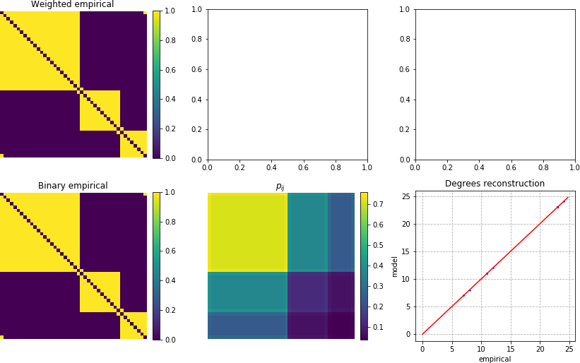
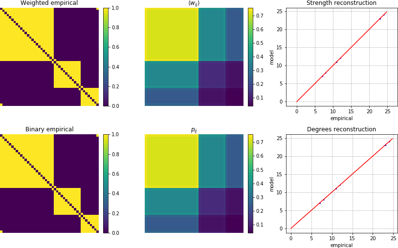
As you can see using the Enhanced Configuration model, both the weights and the link probabilities are correctly fitted in the model, even if this network is unweighted.

Citing

To cite networkqit please include the following publication in BibTeX format:

@article{PhysRevE.98.022322,
  title = {Thermodynamics of network model fitting with spectral entropies},
  author = {Nicolini, Carlo and Vlasov, Vladimir and Bifone, Angelo},
  journal = {Phys. Rev. E},
  volume = {98},
  issue = {2},
  pages = {022322},
  numpages = {10},
  year = {2018},
  month = {Aug},
  publisher = {American Physical Society},
  doi = {10.1103/PhysRevE.98.022322},
  url = {https://link.aps.org/doi/10.1103/PhysRevE.98.022322}
}

It is also vailable at this link

TODO

I would like to find someone helping in implementing XLA instead of autograd as the basic package for automatic differentiation. Indeed XLA has the possibility to extend calculations on the GPU and (in future) on MultiGPU or TPU systems, effortlessly. It would be possible to scale to much larger problems.

CarloNicolini / networkqit