Welcome to qnm

qnm is an open-source Python package for computing the Kerr quasinormal mode frequencies, angular separation constants, and spherical-spheroidal mixing coefficients. The qnm package includes a Leaver solver with the Cook-Zalutskiy spectral approach to the angular sector, and a caching mechanism to avoid repeating calculations.

With this python package, you can compute the QNMs labeled by different (s,l,m,n), at a desired dimensionless spin parameter 0≤a<1. The angular sector is treated as a spectral decomposition of spin-weighted spheroidal harmonics into spin-weighted spherical harmonics. Therefore you get the spherical-spheroidal decomposition coefficients for free when solving for ω and A (see below for details).

We have precomputed a large cache of low-lying modes (s=-2 and s=-1, all l<8, all n<7). These can be automatically installed with a single function call, and interpolated for good initial guesses for root-finding at some value of a.

Installation

PyPI

qnm is available on PyPI:

pip install qnm

Conda

qnm is available on conda-forge:

conda install -c conda-forge qnm

From source

git clone https://github.com/duetosymmetry/qnm.git
cd qnm
python setup.py install

If you do not have root permissions, replace the last step with python setup.py install --user. Instead of using setup.py manually, you can also replace the last step with pip install . or pip install --user ..

Dependencies

All of these can be installed through pip or conda.

numpy
scipy
numba
tqdm (just for qnm.download_data() progress)
pathlib2 (backport of pathlib to pre-3.4 python)

Documentation

Automatically-generated API documentation is available on Read the Docs: qnm.

For a didactic introduction, you can watch my talk at the Spring 2020 BHPToolkit Workshop (starting around 4:11:02 in the stream. You can also follow along with the qnm presentation notebook.

Usage

The highest-level interface is via qnm.cached.KerrSeqCache, which loads cached spin sequences from disk. A spin sequence is just a mode labeled by (s,l,m,n), with the spin a ranging from a=0 to some maximum, e.g. 0.9995. A large number of low-lying spin sequences have been precomputed and are available online. The first time you use the package, download the precomputed sequences:

import qnm

qnm.download_data() # Only need to do this once
# Trying to fetch https://duetosymmetry.com/files/qnm/data.tar.bz2
# Trying to decompress file /<something>/qnm/data.tar.bz2
# Data directory /<something>/qnm/data contains 860 pickle files

Then, use qnm.modes_cache to load a qnm.spinsequence.KerrSpinSeq of interest. If the mode is not available, it will try to compute it (see detailed documentation for how to control that calculation).

grav_220 = qnm.modes_cache(s=-2,l=2,m=2,n=0)
omega, A, C = grav_220(a=0.68)
print(omega)
# (0.5239751042900845-0.08151262363119974j)

Calling a spin sequence seq with seq(a) will return the complex quasinormal mode frequency omega, the complex angular separation constant A, and a vector C of coefficients for decomposing the associated spin-weighted spheroidal harmonics as a sum of spin-weighted spherical harmonics (see below for details).

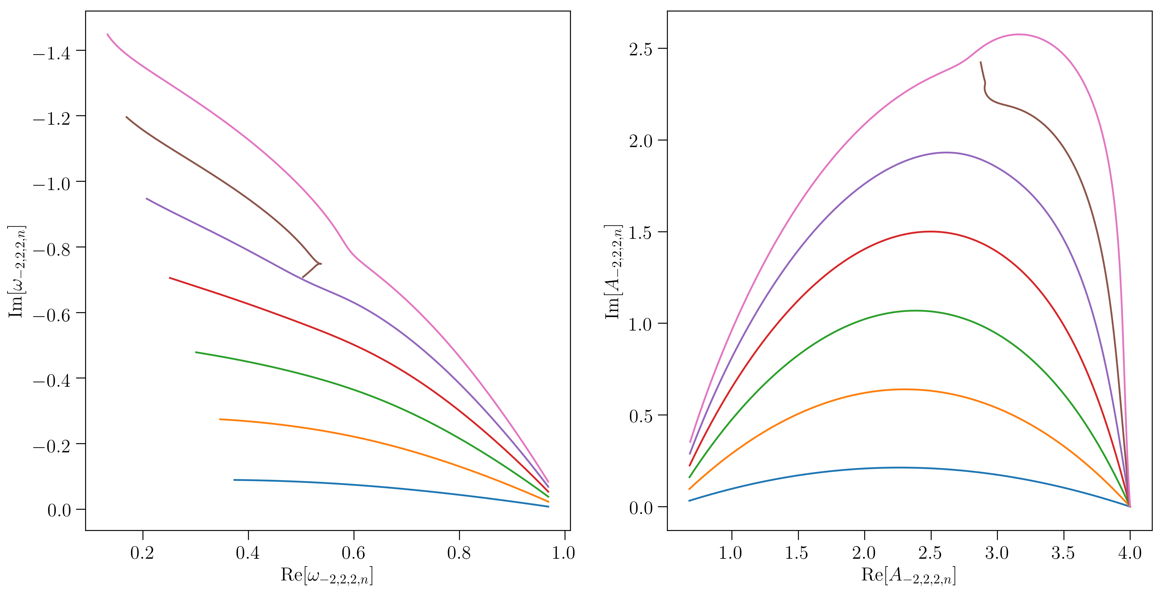
Visual inspections of modes are very useful to check if the solver is behaving well. This is easily accomplished with matplotlib. Here are some partial examples (for the full examples, see the file notebooks/examples.ipynb in the source repo):

import numpy as np
import matplotlib as mpl
import matplotlib.pyplot as plt

s, l, m = (-2, 2, 2)
mode_list = [(s, l, m, n) for n in np.arange(0,7)]
modes = { ind : qnm.modes_cache(*ind) for ind in mode_list }

plt.subplot(1, 2, 1)
for mode, seq in modes.items():
    plt.plot(np.real(seq.omega),np.imag(seq.omega))

plt.subplot(1, 2, 2)
for mode, seq in modes.items():
    plt.plot(np.real(seq.A),np.imag(seq.A))

Which results in the following figure (modulo formatting):

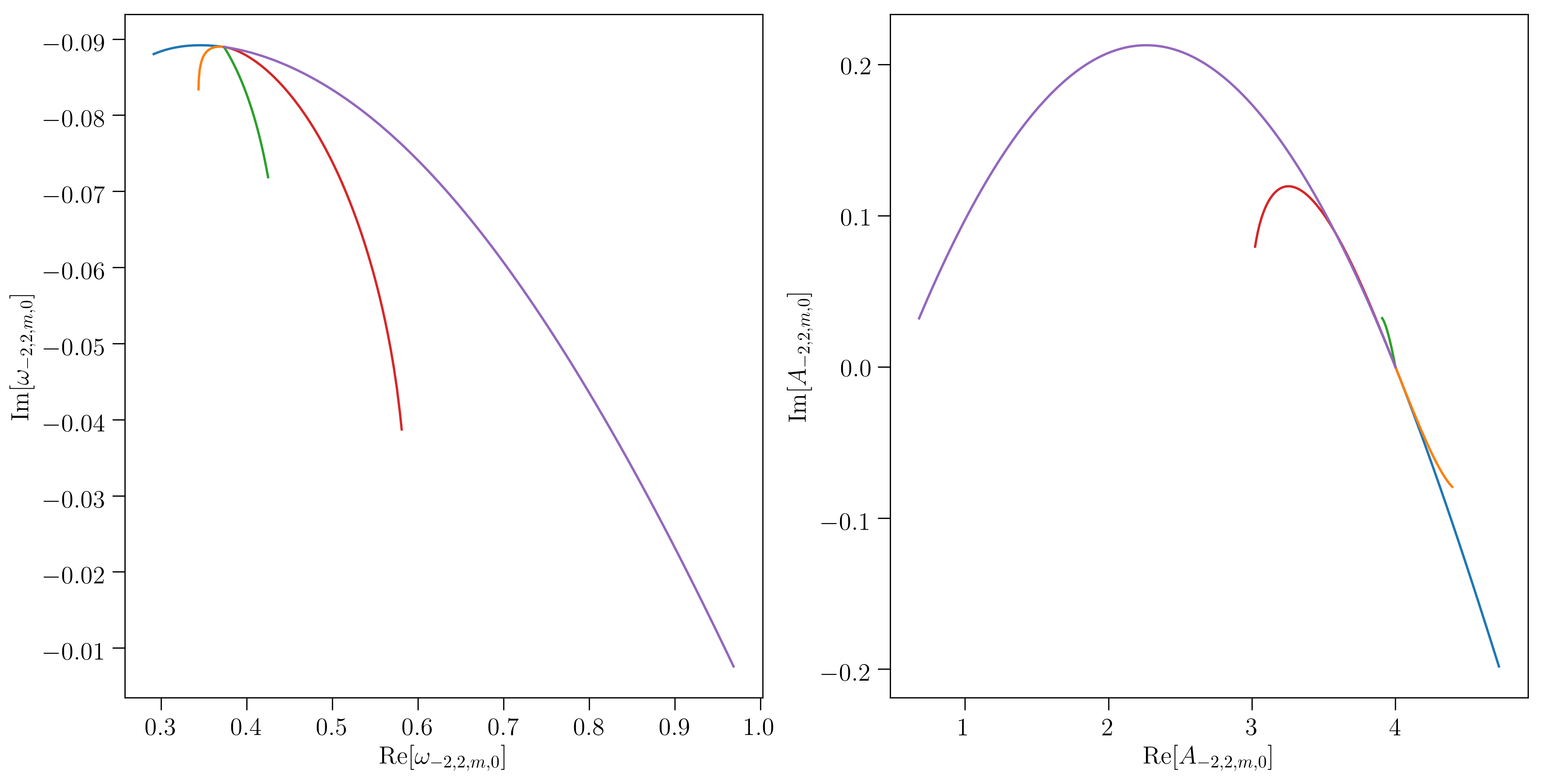
s, l, n = (-2, 2, 0)
mode_list = [(s, l, m, n) for m in np.arange(-l,l+1)]
modes = { ind : qnm.modes_cache(*ind) for ind in mode_list }

plt.subplot(1, 2, 1)
for mode, seq in modes.items():
    plt.plot(np.real(seq.omega),np.imag(seq.omega))

plt.subplot(1, 2, 2)
for mode, seq in modes.items():
    plt.plot(np.real(seq.A),np.imag(seq.A))

Which results in the following figure (modulo formatting):

Precision and validation

The default tolerances for continued fractions, cf_tol, is 1e-10, and for complex root-polishing, tol, is DBL_EPSILON≅1.5e-8. These can be changed at runtime so you can re-polish the cached values to higher precision.

Greg Cook's precomputed data tables (which were computed with arbitrary-precision arithmetic) can be used for validating the results of this code. See the comparison notebook notebooks/Comparison-against-Cook-data.ipynb to see such a comparison, which can be modified to compare any of the available modes.

Spherical-spheroidal decomposition

The angular dependence of QNMs are naturally spin-weighted spheroidal harmonics. The spheroidals are not actually a complete orthogonal basis set. Meanwhile spin-weighted spherical harmonics are complete and orthonormal, and are used much more commonly. Therefore you typically want to express a spheroidal (on the left hand side) in terms of sphericals (on the right hand side),

$equation $${}_s Y_{\\ell m}(\\theta, \\phi; a\\omega) = {\\sum_{\\ell'=\\ell_{\\min} (s,m)}^{\\ell_\\max}} C_{\\ell' \\ell m}(a\\omega)\\ {}_s Y_{\\ell' m}(\\theta, \\phi) \\,.$$$

Here ℓmin=max(|m|,|s|) and ℓmax can be chosen at run time. The C coefficients are returned as a complex ndarray, with the zeroth element corresponding to ℓmin. To avoid indexing errors, you can get the ndarray of ℓ values by calling qnm.angular.ells, e.g.

ells = qnm.angular.ells(s=-2, m=2, l_max=grav_220.l_max)

Contributing

Contributions are welcome! There are at least two ways to contribute to this codebase:

If you find a bug or want to suggest an enhancement, use the issue tracker on GitHub. It's a good idea to look through past issues, too, to see if anybody has run into the same problem or made the same suggestion before.
If you will write or edit the python code, we use the fork and pull request model.

You are also allowed to make use of this code for other purposes, as detailed in the MIT license. For any type of contribution, please follow the code of conduct.

How to cite

If this package contributes to a project that leads to a publication, please acknowledge this by citing the qnm article in JOSS. The following BibTeX entry is available in the qnm.__bibtex__ string:

@article{Stein:2019mop,
      author         = "Stein, Leo C.",
      title          = "{qnm: A Python package for calculating Kerr quasinormal
                        modes, separation constants, and spherical-spheroidal
                        mixing coefficients}",
      journal        = "J. Open Source Softw.",
      volume         = "4",
      year           = "2019",
      number         = "42",
      pages          = "1683",
      doi            = "10.21105/joss.01683",
      eprint         = "1908.10377",
      archivePrefix  = "arXiv",
      primaryClass   = "gr-qc",
      SLACcitation   = "%%CITATION = ARXIV:1908.10377;%%"
}

Credits

The code is developed and maintained by Leo C. Stein.

BlackHolePerturbationToolkit / qnm