| author | level | title | subtitle | beastversion |
|---|---|---|---|---|
Nicola F. Müller |
Professional |
AIM in StarBeast2 v0.15.2 Tutorial |
Inferring species trees and gene flow from multiple loci |
2.5.2 |
BEAST2 (http://www.beast2.org) is a free software package for Bayesian evolutionary analysis of molecular sequences using MCMC and strictly oriented toward inference using rooted, time-measured phylogenetic trees. This tutorial is written for BEAST v{{ page.beastversion }} {% cite BEAST2book2014 --file AIM-Tutorial/master-refs %}.
BEAUti2 is a graphical user interface tool for generating BEAST2 XML configuration files.
Both BEAST2 and BEAUti2 are Java programs, which means that the exact same code runs on all platforms. For us it simply means that the interface will be the same on all platforms. The screenshots used in this tutorial are taken on a Mac OS X computer; however, both programs will have the same layout and functionality on both Windows and Linux. BEAUti2 is provided as a part of the BEAST2 package so you do not need to install it separately.
TreeAnnotator is used to summarise the posterior sample of trees to produce a maximum clade credibility tree. It can also be used to summarise and visualise the posterior estimates of other tree parameters (e.g. node height).
TreeAnnotator is provided as a part of the BEAST2 package so you do not need to install it separately.
Tracer (http://tree.bio.ed.ac.uk/software/tracer) is used to summarise the posterior estimates of the various parameters sampled by the Markov Chain. This program can be used for visual inspection and to assess convergence. It helps to quickly view median estimates and 95% highest posterior density intervals of the parameters, and calculates the effective sample sizes (ESS) of parameters. It can also be used to investigate potential parameter correlations. We will be using Tracer v{{ page.tracerversion }}.
FigTree (http://tree.bio.ed.ac.uk/software/figtree) is a program for viewing trees and producing publication-quality figures. It can interpret the node-annotations created on the summary trees by TreeAnnotator, allowing the user to display node-based statistics (e.g. posterior probabilities). We will be using FigTree v{{ page.figtreeversion }}.
We will be using R to analyze and plot the output of the AIM analysis
Practical: Joint inference of the species history and gene flow of 5 anopheles mosquitos by using AIM and coupled MCMC
{% cite Mueller348391 --file AIM-Tutorial/master-refs.bib %}
In this tutorial, we wil infer the species history of 5 different anopheles mosquitos species by using AIM, which is short for Approximate Isolation with Migration. AIM is part of the StarBeast2 package. This model can be used when we want to jointly infer the species histories for multiple loci and gene flow between extant and ancestral species.
The aim is to:
- Learn how to jointly infer the species tree and gene flow of multiple loci from multiple species
- Get to know how to choose the set-up of such an analysis
- Learn how to process the output of an AIM analysis
The data was previously used to infer the species history of the anopheles gambie complex in {% cite fontaine2015extensive --file AIM-Tutorial/master-refs.bib %}. It is comprised of 27 loci, each of a length of about 1000 bp, from the left arm of the 3rd chromosome.
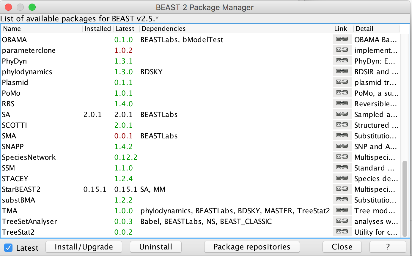
First, we have to download the packages StarBeast2 and CoupledMCMC by using the BEAUTi package manager. Go to File >> Manage Packages and download the package and CoupledMCMC StarBeast2.
Figure 1: Download the StarBeast2 and CoupledMCMC packages.Next, we have to load the BEAUTi template from File, select Template >> AIM.
The sequences for the different loci can be found in the data folder name can be either drag and dropped into BEAUti or imported by Import Alignment. It will ask us what type the data is. If we say nucleotide, it will ask us for each loci individually. Since all loci are nucleotide data, we can choose all are nucleotide. To speed up the setup later, we can press Link Site Models and Link Clock Models
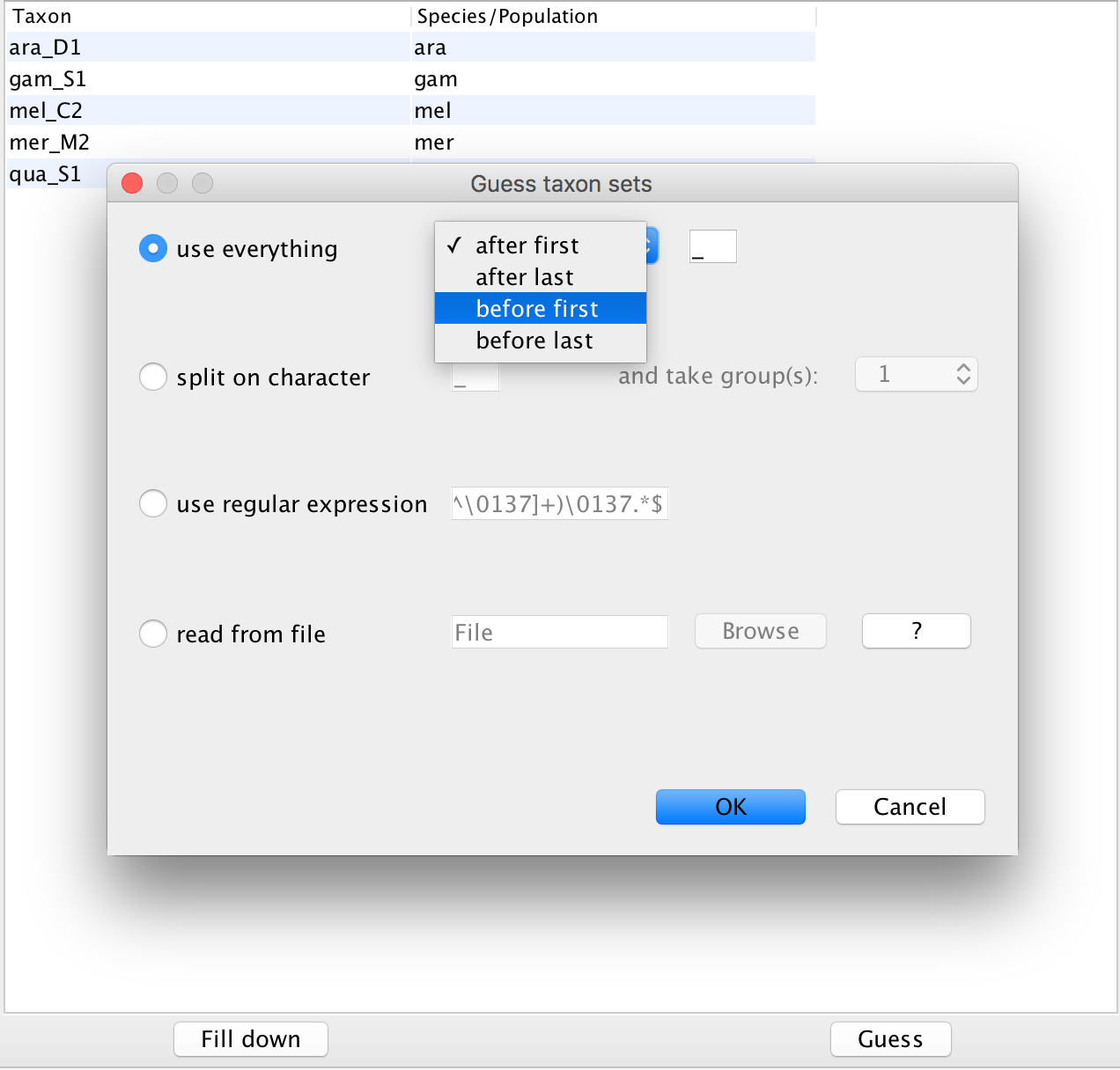
Next, we have to go to the Taxon sets tab. To assign the different individuals to different species, press the Guess button. Use everything before first and press the OK button.
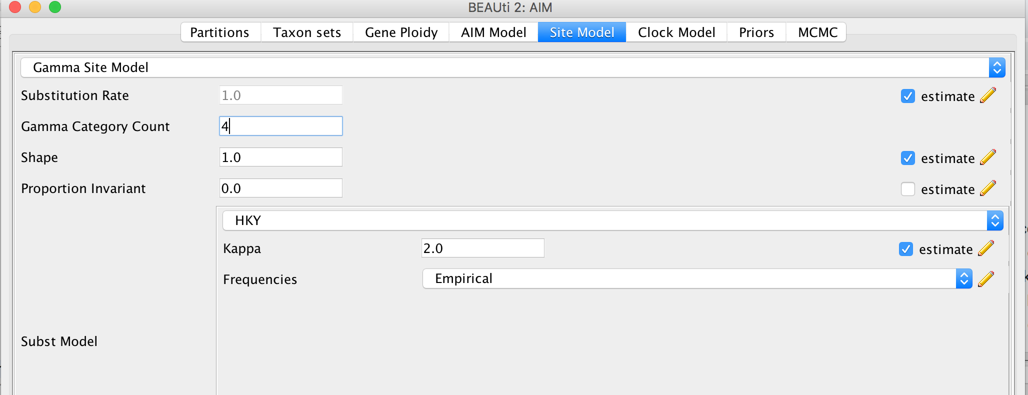
Figure 2: Guess the species of each sampled individual.Since we Linked all the site models of the different loci together when loading the sequence data, we only have to set up the site models once. We will be using an HKY + Γ 4 model that allows for different relative rates of transversions and transitions, as well as for rate hetereogeneity across different sites. Additionally, we should make sure that the estimate button for the substitution rates is clicked to allow for rate variation across different loci. To reduce the number of parameters we have to estimate, we can set frequencies to empirical. After, we can go back to the Partitions field and press Unlink Site Models. Now each loci will have the same site model, but each with different parameters.
Figure 3: Set the site model.Since we have all sequences sampled at the present and no calibration, we do not have any information of time to estimate the clock rate. This means that none of our estimates will be in units of time (e.g. in years), but instead will be in number of substitutions.
The most important priors to specify here are the priors on the number of active routes of gene flow, the rates of gene flow and the effective population sizes. An active route of gene flow denotes a route of gene flow between two species that is non zero. The prior on the number of active routes (migIndicatorSum.species) of gene flow is by defaults a Poisson Prior with lambda=0.693. This puts about 50% of the probability mass on 0 active routes of gene flow. This means that in absence of information about gene flow, a prior probability on having gene flow is fairly low.
In order to speed up the setup, most of the priors are already set to what they should be, expect for the prior on the migration rates. From a hypothetical previous analysis, we know that our tree has a height of about 0.02 substitutions. If we had a migration rate of 1/0.02=50, this would mean that one lineage of a gene from present to the root is expected to migrate on average 1 time. The prior on the migration rates is set in the migRates.Species block. If we set the mean of the log Normal distribution to 2.5, this assumes that we expect about 1 in every 20 lineages to have one migration event over the course of the whole species tree. This is not exactly true, but is an ok approximation for the order of magnitude of how many migration events we expect under this prior.
Figure 4: Setting up the prior on the migration rates.Next, we can save the *.xml file under File >> Save as.
In order to setup the analysis to run with coupled MCMC, we have to open the *.xml and change one line in the xml.
To do so, go to the line with:
<run id="mcmc" spec="MCMC" chainLength="10000000" storeEvery="5000">
To have a run with coupled MCMC, we have to replace the above line with:
<run id="mcmc" spec="beast.coupledMCMC.CoupledMCMC" logHeatedChains="true" chainLength="10000000" storeEvery="5000" deltaTemperature="0.1" chains="2" resampleEvery="10000">
-
logHeatedChains="true"logs the log files of the heated chains if true. -
chainLength="100000000"defines for how many iterations the chains is run -
deltaTemperature="0.1"defines the temperature difference between the chain n and chain n-1. -
chains="2"defines the number of parallel chains that are run. The first chain is the one that explores the posterior just like a normal MCMC chain. All other chains are what's called heated. This means that MCMC moves of those chains have a higher probability of being accepted. While these heated chains don't explore the posterior properly, they can be used to propose new states to the one cold chain.
The output to the screen of a Coupled MCMC run looks slightly different then the one of a standard MCMC run. The column called sample describes at which iteration of the coupled MCMC we are. The column swapsColdChain denotes how many times the one cold chain (the chain that runs just like a regular MCMC chain) has been swapped with another chain. The swapProbability denotes how likely it is that a swapping between two chains is accepted. This vaue should be somewhere between 0.2 and 0.6. A low values indicates that the heated chains are running too hot and are not efficiently exploring the posterior. A too high values indicates that the heated chains are not running hot enough and are thus exploring parameter space that are too similar to the one of the cold chain.
sample    swapsColdCain    swapProbability
10000    0    0.0 --
20000    1    0.5 3m15s/Msamples
30000    1    0.3333333333333333 2m56s/Msamples
40000    1    0.25 2m34s/Msamples
50000    1    0.2 2m29s/Msamples
60000    1    0.16666666666666666 2m24s/Msamples
70000    1    0.14285714285714285 2m22s/Msamples
80000    1    0.125 2m20s/Msamples
90000    1    0.1111111111111111 2m15s/Msamples
100000    1    0.1 2m12s/Msamples
110000    1    0.09090909090909091 2m9s/Msamples
120000    1    0.08333333333333333 2m8s/Msamples
The webpage https://darrenjw.wordpress.com/2013/09/29/parallel-tempering-and-metropolis-coupled-mcmc/, gives a good introduction on how coupled MCMC works.
Run the *.xml using BEAST2 or use finished runs from the precooked-runs folder. The analysis should take about 10 to 20 minutes.
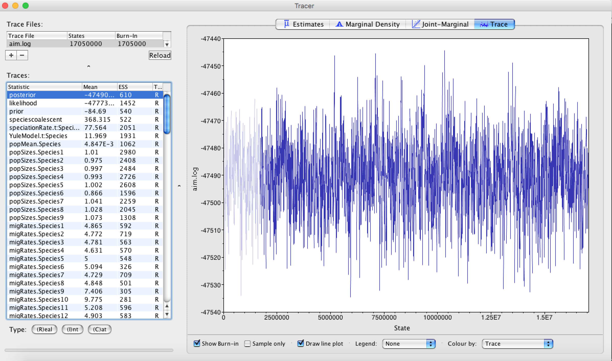
First, we can open the aim.log file in tracer to check if the MCMC has converged. The ESS value should be above 200 for almost all values and especially for the posterior estimates. The burnin taken by Tracer is 10%, but for this analysis 1% is enough.
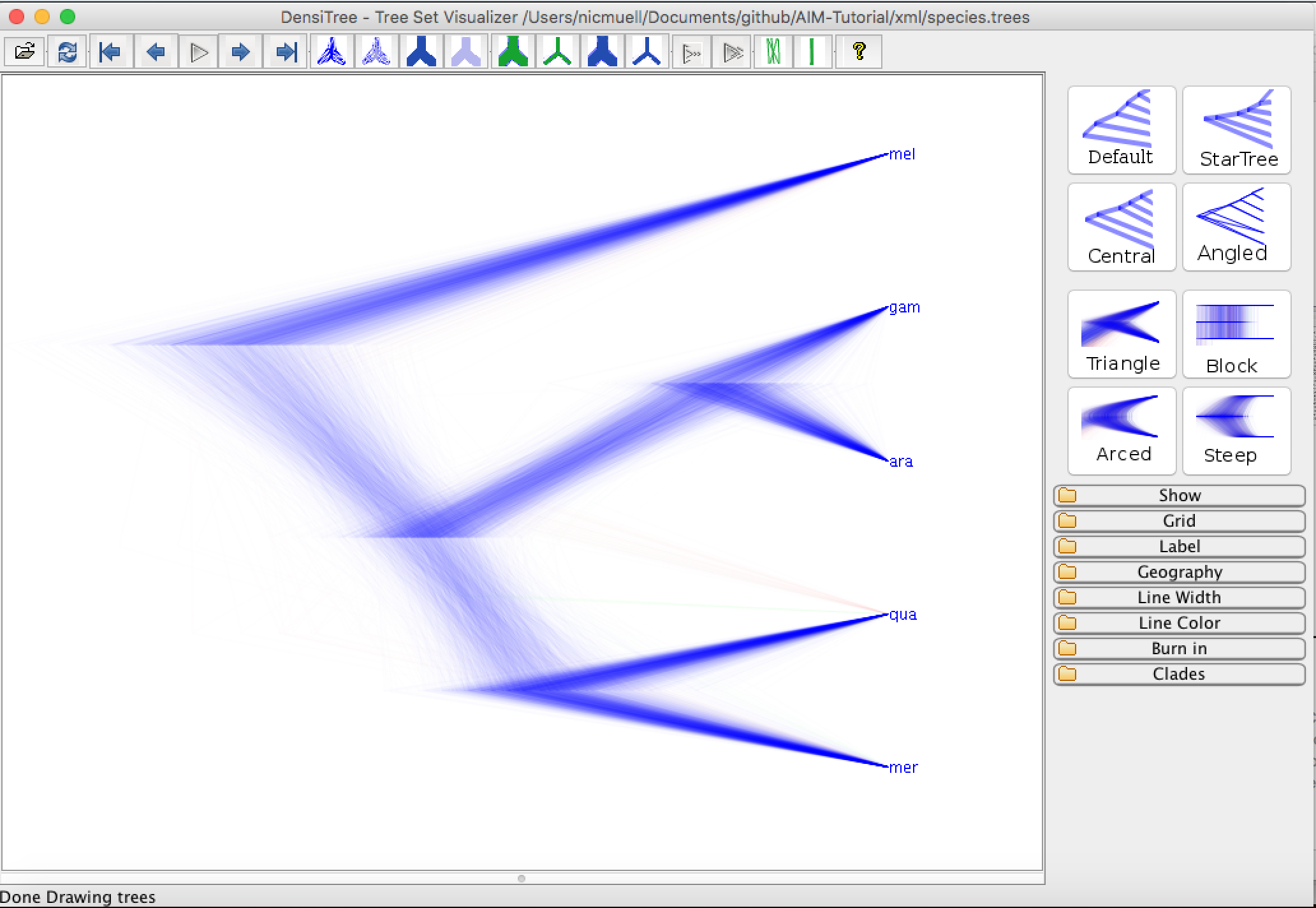
First, we can have a look at the distribution of species trees in DensiTree. To do so, open the files species.trees in DensiTree.
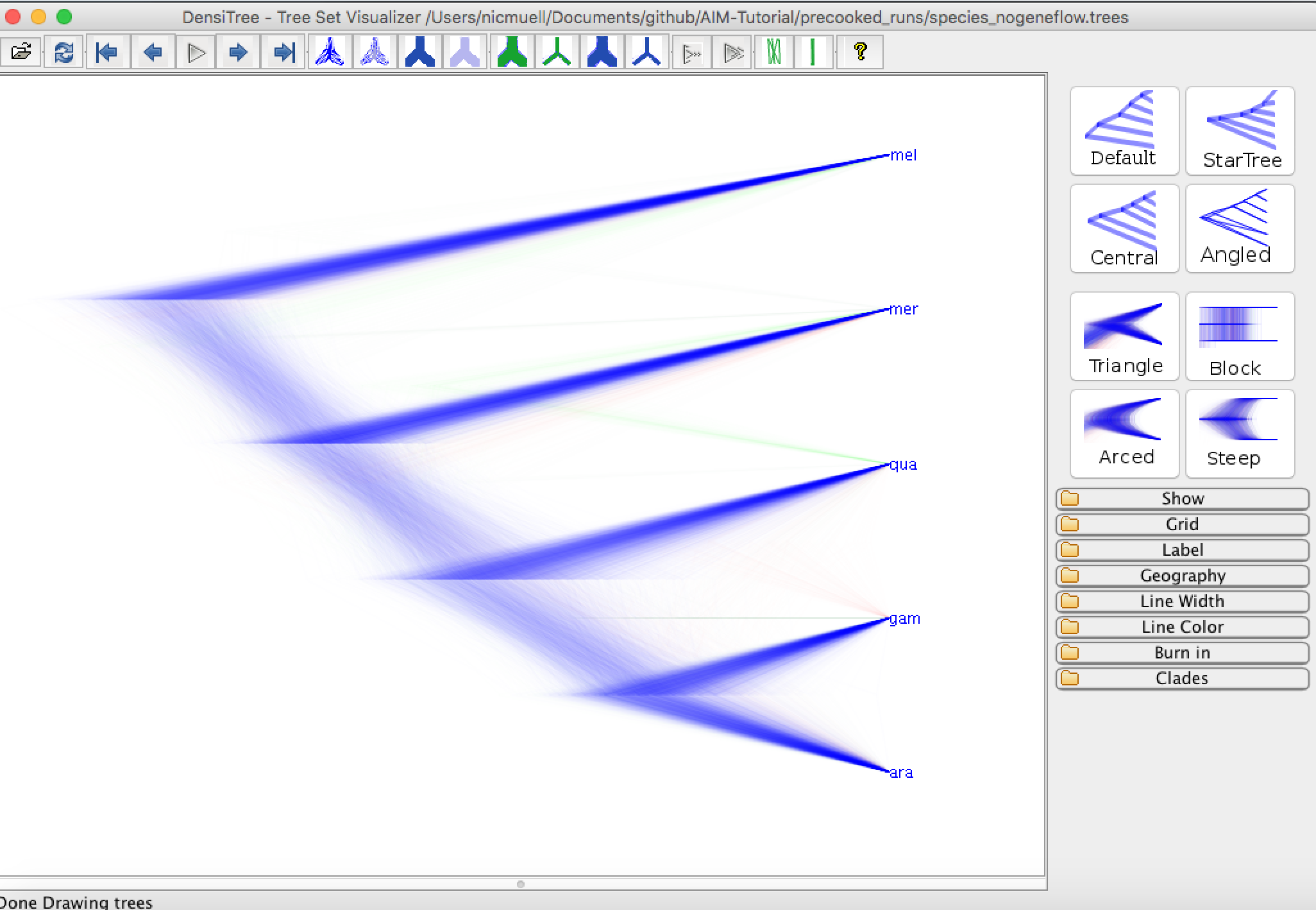
We can now compare the distribution of species trees inferred under AIM to the case when we don't have any gene flow. This file can be found in the pre-cooked runs folder and is called species_nogeneflow.trees
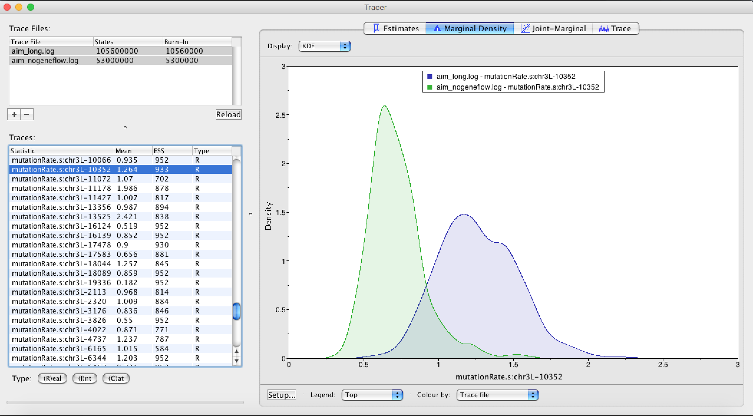
Next, we can check which which genes most likely drive these differences. In order to do so, we can compare inferred relative rates of evolution for every loci between runs with and runs without gene flow. To do so, we can load the two files aim.log and aim_nogeneflow.log in tracer. When we compare the relative rates of mutation between most loci, they look fairly similar between with and without gene flow. Locus nr 10352 however has a very different inferred mutation rate, indicating that there is something different going on in that loci depending on wether we allow for gene flow or not.
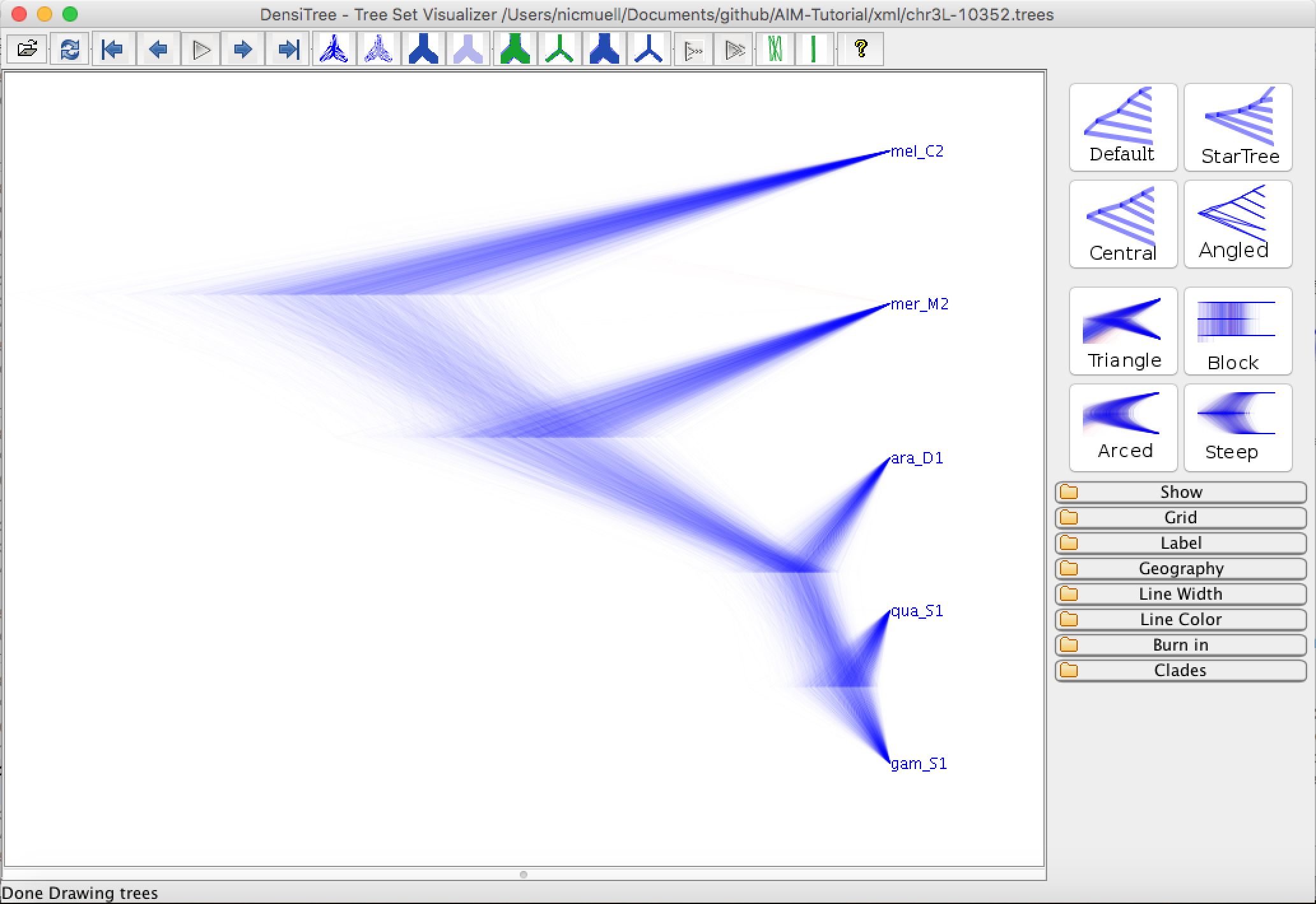
Next, we can open the inferred tree of locus 10352 when accounting for gene flow in DensiTree
Figure 9: Inferred gene tree of chr3L-10352.In AIM, the attachement of An. quadriannulatus is explained by gene flow. When not accounting for gene flow, this causes the topology of the species tree to be slightly different by essentially pushing the attachment of An. quadriannulatus closer to An. gambia. We will next analyse between which species there was gene flow by using an R script.
The analysis script for the analysis of the species tree can be found in the scripts folder. The R script analyseAIMrun.R can be used to analyse AIM runs and to plot species trees and the gene flow between species. First, we'll need to install a few R packages for the script to run. To do so, open R and then type in the follwing few lines:
install.packages("devtools", type = "source")
devtools::install_github("thibautjombart/OutbreakTools")
install.packages("ggplot2", type = "source")
install.packages("phytools", type = "source")
install.packages("ape", type = "source")
install.packages("ggtree", type = "source")
devtools is needed to install OutbreakTools.
OutbreakTools is needed to read in node annotated trees.
ggplot2 and ggtree are needed to plot trees and phytools and ape are needed to analyse node heights etc.
Running analyseAIMrun.R will take the tree file specified in the line:
trees <- "./../precooked_runs/species_long.trees
as intput. If you want to use a different species.trees files, this line has to be changed. Next, we can try to run the script. If the error Error in start:end : NA/NaN argument appears, the last line of the *.trees file we were using was probably not End;. The function that reads in the trees into R however requires this to be the case. The easiest way to avoid this error is therefore to just add End; to the *.trees file in a TextEditor. Otherwise, running logCombiner on the *.trees file will resolve the error as well. Running the script will then read in the node annotated trees and take a burnin as specified in the line burn_in = 0.1. It will then count how many different unique ranked tree topologies there are. This means that the script distinguished between trees that have the same topology but where the ordering of internal nodes is different. This has to be done in AIM, since each ranked topologies has a different set of co-existing species. This means that the meaning of parameters is different for each of these different topologies.
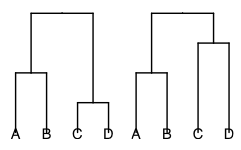
The script will produce one figure and one log file for each of the uniquely ranked species tree topologies. Uniquely ranked tree topologies distinguishes between trees with the same topology, but different order of nodes.
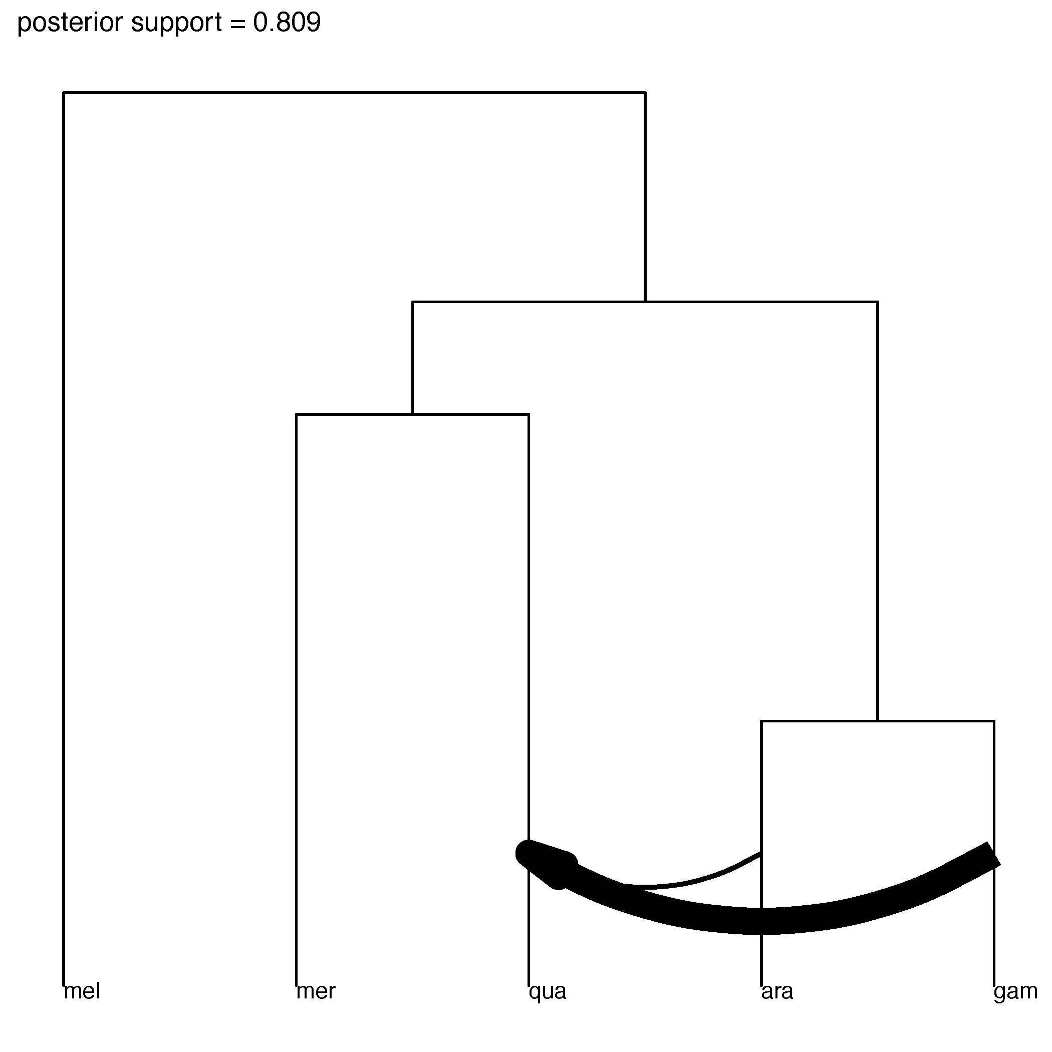
Figure 10: Tree with the same topology but different node order.The figure shows the species tree as well as between which species gene flow is supported. Only if gene flow is supported with Bayes Factor with more than 20, it is plotted. The log file reports the parameter estimates seperately for each of the different uniquely ranked species tree topologies. The files are numbered by their relative posterior support, with file nr 1 being the most probable species tree. The support for each individual ranked topolofy is given as the title of each figure.
The figure of the most probable inferred tree should look something like the figure below.
Figure 11: Most probable ranked tree topology.Meaning that we infer gene flow to be probable from An. gambia to An. quadriannulatus.
- Different priors, especially on how much and how strong gene flow is expected to occur, can have a large impact on the species tree that is inferred. The reason is that in a IM model, coalescent events on a gene between two species can either be explained by gene flow or by a speciation event.
- Variation in the data that is not accounted for by the model can lead to wrong estimates of the species tree or between which species gene flow occurs.
- Jointly inferring the species tree, gene flow, effective population sizes, gene trees and evolutionary models can take a long time.
- AIM source code: https://github.com/genomescale/starbeast2
- Bayesian Evolutionary Analysis with BEAST 2 {% cite BEAST2book2014 --file AIM-Tutorial/master-refs.bib %}
- BEAST 2 website and documentation: http://www.beast2.org/
- Join the BEAST user discussion: http://groups.google.com/group/beast-users
{% bibliography --cited --file AIM-Tutorial/master-refs %}
