coronavirus 
![]()
![]()

The coronavirus package provides a tidy format dataset of the 2019 Novel Coronavirus COVID-19 (2019-nCoV) epidemic and the vaccination efforts by country. The raw data is being pulled from the Johns Hopkins University Center for Systems Science and Engineering (JHU CCSE) Coronavirus repository.
More details available
here, and a csv format
of the package dataset available
here

Important Notes
- As this an ongoing situation, frequent changes in the data format may occur, please visit the package changelog (e.g., News) and/or see pinned issues to get updates about those changes
- As of Auguest 4th JHU CCSE stopped track recovery cases, please see this issue for more details
- Negative values and/or anomalies may occurred in the data for the
following reasons:
- The calculation of the daily cases from the raw data which is in cumulative format is done by taking the daily difference. In some cases, some retro updates not tie to the day that they actually occurred such as removing false positive cases
- Anomalies or error in the raw data
- Please see this issue for more details
Vignettes
Additional documentation available on the followng vignettes:
- Introduction to the Coronavirus Dataset
- Covid19R Project Data Format
- Update the coronavirus Dataset
- Covid19 Vaccine Data
- Geospatial Visualization
Installation
Install the CRAN version:
install.packages("coronavirus")Install the Github version (refreshed on a daily bases):
# install.packages("devtools")
devtools::install_github("RamiKrispin/coronavirus")
Datasets
The package provides the following two datasets:
-
coronavirus - tidy (long) format of the JHU CCSE datasets. That includes the following columns:
date- The date of the observation, usingDateclassprovince- Name of province/state, for countries where data is provided split across multiple provinces/statescountry- Name of country/regionlat- The latitude codelong- The longitude codetype- An indicator for the type of cases (confirmed, death, recovered)cases- Number of cases on given dateuid- Country codeprovince_state- Province or state if applicableiso2- Officially assigned country code identifiers with two-letteriso3- Officially assigned country code identifiers with three-lettercode3- UN country codefips- Federal Information Processing Standards code that uniquely identifies counties within the USAcombined_key- Country and province (if applicable)population- Country or province populationcontinent_name- Continent namecontinent_code- Continent code
-
covid19_vaccine - a tidy (long) format of the the Johns Hopkins Centers for Civic Impact global vaccination dataset by country. This dataset includes the following columns:
country_region- Country or region namedate- Data collection date in YYYY-MM-DD formatdoses_admin- Cumulative number of doses administered. When a vaccine requires multiple doses, each one is counted independentlypeople_partially_vaccinated- Cumulative number of people who received at least one vaccine dose. When the person receives a prescribed second dose, it is not counted twicepeople_fully_vaccinated- Cumulative number of people who received all prescribed doses necessary to be considered fully vaccinatedreport_date_string- Data report date in YYYY-MM-DD formatuid- Country codeprovince_state- Province or state if applicableiso2- Officially assigned country code identifiers with two-letteriso3- Officially assigned country code identifiers with three-lettercode3- UN country codefips- Federal Information Processing Standards code that uniquely identifies counties within the USAlat- Latitudelong- Longitudecombined_key- Country and province (if applicable)population- Country or province populationcontinent_name- Continent namecontinent_code- Continent code
Data refresh
While the coronavirus CRAN
version is updated
every month or two, the Github (Dev)
version is updated on a
daily bases. The update_dataset function enables to overcome this gap
and keep the installed version with the most recent data available on
the Github version:
library(coronavirus)
update_dataset()
Note: must restart the R session to have the updates available
Alternatively, you can pull the data using the
Covid19R project data
standard
format
with the refresh_coronavirus_jhu function:
covid19_df <- refresh_coronavirus_jhu()
head(covid19_df)
#>         date    location location_type location_code location_code_type  data_type value      lat      long
#> 1 2021-10-04 Afghanistan       country            AF         iso_3166_2 deaths_new     6 33.93911 67.709953
#> 2 2021-10-03 Afghanistan       country            AF         iso_3166_2 deaths_new     0 33.93911 67.709953
#> 3 2020-11-09 Afghanistan       country            AF         iso_3166_2 deaths_new     6 33.93911 67.709953
#> 4 2021-10-10 Afghanistan       country            AF         iso_3166_2 deaths_new     4 33.93911 67.709953
#> 5 2021-10-06 Afghanistan       country            AF         iso_3166_2 deaths_new     6 33.93911 67.709953
#> 6 2020-11-10 Afghanistan       country            AF         iso_3166_2 deaths_new    12 33.93911 67.709953
Usage
data("coronavirus")

head(coronavirus)
#>         date province country     lat      long      type cases
#> 1 2020-01-22  Alberta  Canada 53.9333 -116.5765 confirmed     0
#> 2 2020-01-23  Alberta  Canada 53.9333 -116.5765 confirmed     0
#> 3 2020-01-24  Alberta  Canada 53.9333 -116.5765 confirmed     0
#> 4 2020-01-25  Alberta  Canada 53.9333 -116.5765 confirmed     0
#> 5 2020-01-26  Alberta  Canada 53.9333 -116.5765 confirmed     0
#> 6 2020-01-27  Alberta  Canada 53.9333 -116.5765 confirmed     0
Summary of the total confrimed cases by country (top 20):
library(dplyr)

summary_df <- coronavirus %>%
  filter(type == "confirmed") %>%
  group_by(country) %>%
  summarise(total_cases = sum(cases)) %>%
  arrange(-total_cases)

summary_df %>% head(20)
#> # A tibble: 20 × 2
#>    country        total_cases
#>    <chr>                <int>
#>  1 US                44683014
#>  2 India             34020730
#>  3 Brazil            21597949
#>  4 United Kingdom     8311851
#>  5 Russia             7742899
#>  6 Turkey             7540193
#>  7 France             7164924
#>  8 Iran               5742083
#>  9 Argentina          5268653
#> 10 Spain              4980206
#> 11 Colombia           4975656
#> 12 Italy              4707087
#> 13 Germany            4343591
#> 14 Indonesia          4231046
#> 15 Mexico             3732429
#> 16 Poland             2928065
#> 17 South Africa       2913880
#> 18 Ukraine            2697176
#> 19 Philippines        2690455
#> 20 Malaysia           2361529
Summary of new cases during the past 24 hours by country and type (as of 2021-10-13):
library(tidyr)

coronavirus %>%
  filter(date == max(date)) %>%
  select(country, type, cases) %>%
  group_by(country, type) %>%
  summarise(total_cases = sum(cases)) %>%
  pivot_wider(names_from = type,
              values_from = total_cases) %>%
  arrange(-confirmed)
#> # A tibble: 195 × 4
#> # Groups:   country [195]
#>    country        confirmed death recovered
#>    <chr>              <int> <int>     <int>
#>  1 US                120321  3054        NA
#>  2 United Kingdom     41669   136        NA
#>  3 Turkey             31248   236        NA
#>  4 Russia             27926   962        NA
#>  5 India              18987   246        NA
#>  6 Ukraine            17100   493        NA
#>  7 Romania            15733   390        NA
#>  8 Germany            12317    14        NA
#>  9 Iran               12298   194        NA
#> 10 Thailand           10064    82        NA
#> 11 Malaysia            7950    68        NA
#> 12 Brazil              7852   176        NA
#> 13 Philippines         7083   173        NA
#> 14 Serbia              6699    51        NA
#> 15 Georgia             4837    26        NA
#> 16 Netherlands         3772    13        NA
#> 17 Belgium             3667    13        NA
#> 18 Vietnam             3461   106        NA
#> 19 Bulgaria            3327    98        NA
#> 20 Singapore           3190     9        NA
#> 21 Cameroon            3003    33        NA
#> 22 Italy               2769    37        NA
#> 23 Spain               2758    42        NA
#> 24 Australia           2744    18        NA
#> 25 Lithuania           2740    26        NA
#> 26 Canada              2706    79        NA
#> 27 Poland              2640    40        NA
#> 28 Austria             2614    15        NA
#> 29 Slovakia            2406    20        NA
#> 30 Cuba                2354    28        NA
#> 31 Greece              2312    31        NA
#> 32 Latvia              2236    17        NA
#> 33 Kazakhstan          2084    35        NA
#> 34 Belarus             2060    17        NA
#> 35 Moldova             2052    29        NA
#> 36 Ireland             2051    26        NA
#> 37 Croatia             2022    27        NA
#> 38 Korea, South        1937    13        NA
#> 39 Mongolia            1920    15        NA
#> 40 Iraq                1766    35        NA
#> # … with 155 more rows
Plotting daily confirmed and death cases in Brazil:
library(plotly)

coronavirus %>%
  group_by(type, date) %>%
  summarise(total_cases = sum(cases)) %>%
  pivot_wider(names_from = type, values_from = total_cases) %>%
  arrange(date) %>%
  mutate(active = confirmed - death - recovered) %>%
  mutate(active_total = cumsum(active),
                recovered_total = cumsum(recovered),
                death_total = cumsum(death)) %>%
  plot_ly(x = ~ date,
                  y = ~ active_total,
                  name = 'Active',
                  fillcolor = '#1f77b4',
                  type = 'scatter',
                  mode = 'none',
                  stackgroup = 'one') %>%
  add_trace(y = ~ death_total,
             name = "Death",
             fillcolor = '#E41317') %>%
  add_trace(y = ~recovered_total,
            name = 'Recovered',
            fillcolor = 'forestgreen') %>%
  layout(title = "Distribution of Covid19 Cases Worldwide",
         legend = list(x = 0.1, y = 0.9),
         yaxis = list(title = "Number of Cases"),
         xaxis = list(title = "Source: Johns Hopkins University Center for Systems Science and Engineering"))
Plot the confirmed cases distribution by counrty with treemap plot:
conf_df <- coronavirus %>%
  filter(type == "confirmed") %>%
  group_by(country) %>%
  summarise(total_cases = sum(cases)) %>%
  arrange(-total_cases) %>%
  mutate(parents = "Confirmed") %>%
  ungroup()

  plot_ly(data = conf_df,
          type= "treemap",
          values = ~total_cases,
          labels= ~ country,
          parents=  ~parents,
          domain = list(column=0),
          name = "Confirmed",
          textinfo="label+value+percent parent")
data(covid19_vaccine)

head(covid19_vaccine)
#>   country_region       date doses_admin people_partially_vaccinated people_fully_vaccinated report_date_string uid province_state iso2 iso3 code3 fips      lat      long combined_key population
#> 1    Afghanistan 2021-02-22           0                           0                       0         2021-02-22   4           <NA>   AF  AFG     4 <NA> 33.93911 67.709953  Afghanistan   38928341
#> 2    Afghanistan 2021-02-23           0                           0                       0         2021-02-23   4           <NA>   AF  AFG     4 <NA> 33.93911 67.709953  Afghanistan   38928341
#> 3    Afghanistan 2021-02-24           0                           0                       0         2021-02-24   4           <NA>   AF  AFG     4 <NA> 33.93911 67.709953  Afghanistan   38928341
#> 4    Afghanistan 2021-02-25           0                           0                       0         2021-02-25   4           <NA>   AF  AFG     4 <NA> 33.93911 67.709953  Afghanistan   38928341
#> 5    Afghanistan 2021-02-26           0                           0                       0         2021-02-26   4           <NA>   AF  AFG     4 <NA> 33.93911 67.709953  Afghanistan   38928341
#> 6    Afghanistan 2021-02-27           0                           0                       0         2021-02-27   4           <NA>   AF  AFG     4 <NA> 33.93911 67.709953  Afghanistan   38928341
#>   continent_name continent_code
#> 1           Asia             AS
#> 2           Asia             AS
#> 3           Asia             AS
#> 4           Asia             AS
#> 5           Asia             AS
#> 6           Asia             AS
Plot the top 20 vaccinated countries:
covid19_vaccine %>%
  filter(date == max(date),
         !is.na(population)) %>%
  mutate(fully_vaccinated_ratio = people_fully_vaccinated / population) %>%
  arrange(- fully_vaccinated_ratio) %>%
  slice_head(n = 20) %>%
  arrange(fully_vaccinated_ratio) %>%
  mutate(country = factor(country_region, levels = country_region)) %>%
  plot_ly(y = ~ country,
          x = ~ round(100 * fully_vaccinated_ratio, 2),
          text = ~ paste(round(100 * fully_vaccinated_ratio, 1), "%"),
          textposition = 'auto',
          orientation = "h",
          type = "bar") %>%
  layout(title = "Percentage of Fully Vaccineted Population - Top 20 Countries",
         yaxis = list(title = ""),
         xaxis = list(title = "Source: Johns Hopkins Centers for Civic Impact",
                      ticksuffix = "%"))

Dashboard
Note: Currently, the dashboard is under maintenance due to recent changes in the data structure. Please see this issue
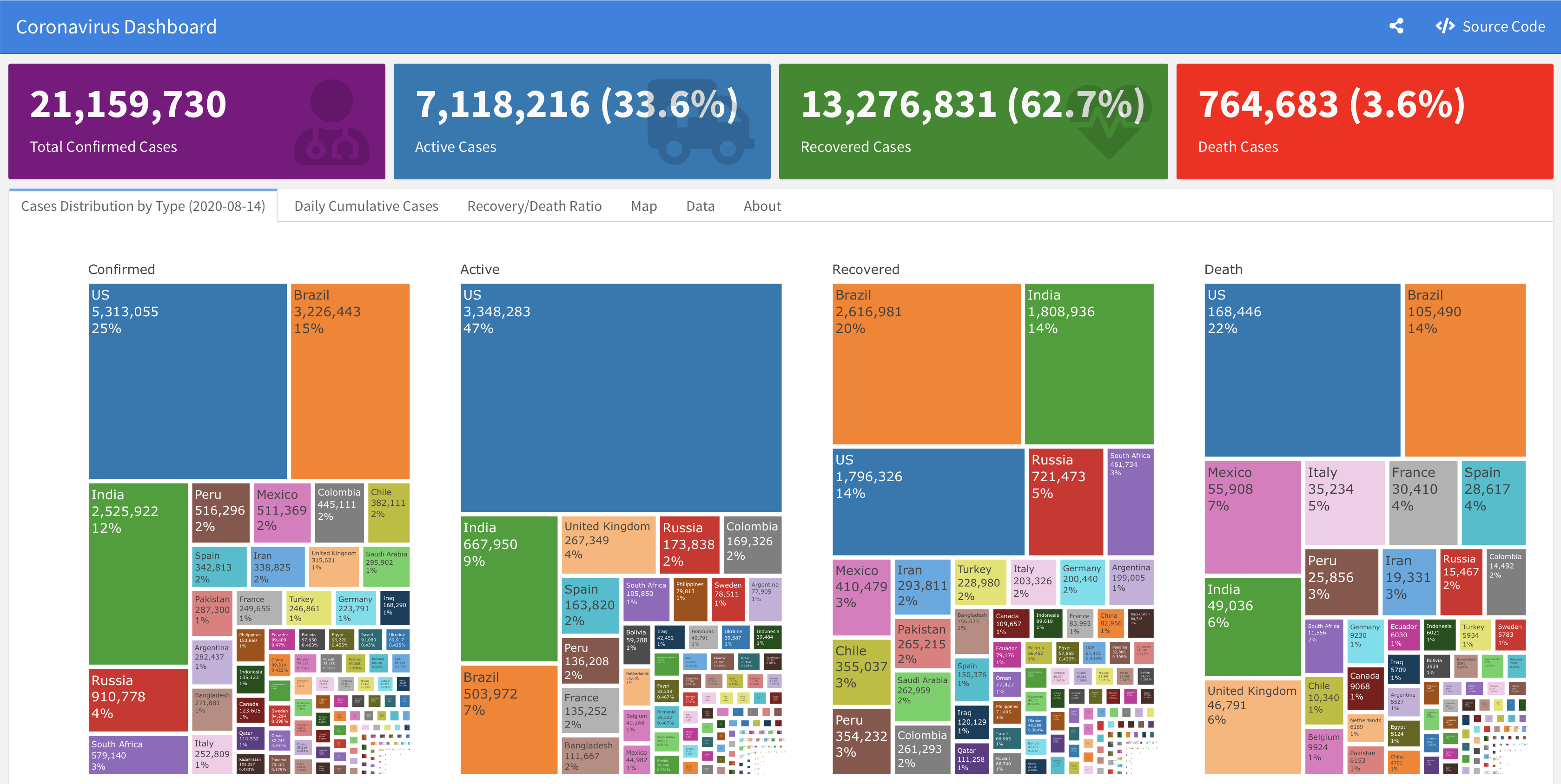
A supporting dashboard is available here
Data Sources
The raw data pulled and arranged by the Johns Hopkins University Center for Systems Science and Engineering (JHU CCSE) from the following resources:
- World Health Organization (WHO): https://www.who.int/
- DXY.cn. Pneumonia. 2020.
https://ncov.dxy.cn/ncovh5/view/pneumonia.
- BNO News:
https://bnonews.com/index.php/2020/04/the-latest-coronavirus-cases/
- National Health Commission of the People’s Republic of China (NHC):
http:://www.nhc.gov.cn/xcs/yqtb/list_gzbd.shtml - China CDC (CCDC):
http:://weekly.chinacdc.cn/news/TrackingtheEpidemic.htm
- Hong Kong Department of Health:
https://www.chp.gov.hk/en/features/102465.html
- Macau Government: https://www.ssm.gov.mo/portal/
- Taiwan CDC:
https://sites.google.com/cdc.gov.tw/2019ncov/taiwan?authuser=0
- US CDC: https://www.cdc.gov/coronavirus/2019-ncov/index.html
- Government of Canada:
https://www.canada.ca/en/public-health/services/diseases/2019-novel-coronavirus-infection/symptoms.html
- Australia Government Department of
Health:https://www.health.gov.au/news/health-alerts/novel-coronavirus-2019-ncov-health-alert
- European Centre for Disease Prevention and Control (ECDC): https://www.ecdc.europa.eu/en/geographical-distribution-2019-ncov-cases
- Ministry of Health Singapore (MOH): https://www.moh.gov.sg/covid-19
- Italy Ministry of Health: https://www.salute.gov.it/nuovocoronavirus
- 1Point3Arces: https://coronavirus.1point3acres.com/en
- WorldoMeters: https://www.worldometers.info/coronavirus/
- COVID Tracking Project: https://covidtracking.com/data. (US Testing and Hospitalization Data. We use the maximum reported value from “Currently” and “Cumulative” Hospitalized for our hospitalization number reported for each state.)
- French Government: https://dashboard.covid19.data.gouv.fr/
- COVID Live (Australia): https://covidlive.com.au/
- Washington State Department of Health:https://www.doh.wa.gov/Emergencies/COVID19
- Maryland Department of Health: https://coronavirus.maryland.gov/
- New York State Department of Health: https://health.data.ny.gov/Health/New-York-State-Statewide-COVID-19-Testing/xdss-u53e/data
- NYC Department of Health and Mental Hygiene: https://www1.nyc.gov/site/doh/covid/covid-19-data.page and https://github.com/nychealth/coronavirus-data
- Florida Department of Health Dashboard: https://services1.arcgis.com/CY1LXxl9zlJeBuRZ/arcgis/rest/services/Florida_COVID19_Cases/FeatureServer/0 and https://fdoh.maps.arcgis.com/apps/opsdashboard/index.html#/8d0de33f260d444c852a615dc7837c86
- Palestine (West Bank and Gaza): https://corona.ps/details
- Israel: https://govextra.gov.il/ministry-of-health/corona/corona-virus/
- Colorado: https://covid19.colorado.gov/data)