The Iris dataset that we got by extracting using R is a well-known dataset in the field of machine learning, often used for demonstrating classification algorithms. It contains measurements of three different species of iris flowers (setosa, versicolor, and virginica) with four features: sepal length, sepal width, petal length, and petal width. The goal of this project is to build a classification model using PySpark's MLlib to accurately predict the species of an iris flower based on these measurements.
- Extract the Iris dataset from R
- Load the Iris dataset into a Spark DataFrame.
- Split the dataset into training and testing sets.
- Select and implement a classification algorithm using Spark MLlib.
- Employ techniques such as cross-validation and grid search to fine-tune hyperparameters.
- Evaluate the performance of the tuned model using relevant evaluation metrics (accuracy, precision, recall, F1-score).
Running the Code Inside Putty
We are learning Apache Spark to explore Machine Learning concepts and applications. For this purpose, we are using PuTTY.
from pyspark.sql import SparkSession
from pyspark import SparkContext, SparkConf
from pyspark.ml.feature import StringIndexer, VectorAssembler
from pyspark.ml.classification import RandomForestClassifier
from pyspark.ml.evaluation import MulticlassClassificationEvaluator
from pyspark.ml.tuning import CrossValidator, ParamGridBuilder

# Initialize Spark context and session
conf = SparkConf().setAppName("Iris Classification")
sc = SparkContext(conf=conf)
spark = SparkSession(sc)

# Load the Iris dataset
iris_data = spark.read.csv("file:///home/maria_dev/azlin/iris.csv", header=True, inferSchema=True)

# Rename the columns to mathc feature names
iris_data = iris_data.withColumnRenamed("Sepal.Length","sepalLength")\
                  .withColumnRenamed("Sepal.Width","sepalWidth")\
                  .withColumnRenamed("Petal.Length","petalLength")\
                  .withColumnRenamed("Petal.Width","petalWidth")\
                  .withColumnRenamed("Species","label")

# Index labels (convert string labels to numeric)
indexer = StringIndexer(inputCol="label", outputCol="indexedLabel").fit(iris_data)
iris_data = indexer.transform(iris_data)

# Verify the label indexing
label_to_index = {row['label']: row['indexedLabel'] for row in iris_data.select("label", "indexedLabel").distinct().collect()}
print("Label to Index Mapping:", label_to_index)

# Assemble features into a feature vector
assembler = VectorAssembler(inputCols=["sepalLength","sepalWidth","petalLength","petalWidth"], outputCol="features")
iris_data = assembler.transform(iris_data)

# Show the first 5 rows
iris_data.show(5)

# Print
iris_data.printSchema()
In Iris dataset, the label column contains string values such as "setosa", "versicolor", and "virginica". These are categorical labels that need to be converted to numeric indices so that they can be processed by the machine learning model more efficiently.
Above output shows 'setosa' was indexed as 2.0, 'versicolor' as 0.0, and 'virginica' as 1.0.
Random Forest
Random Forest handles multiclass classification well, captures non-linear relationships, provides insights into feature importance, and is less prone to overfitting due to its ensemble nature. The Iris dataset is a classic example of a multiclass classification problem with three classes (setosa, versicolor, and virginica) and Random Forest is well-suited for handling multiclass classification tasks effectively.
# Split the dataset into training and testing sets
train_data, test_data = iris_data.randomSplit([0.8,0.2], seed=42)

# Random Forest is selected as a classification algorithm
randomForest = RandomForestClassifier(labelCol="indexedLabel", featuresCol="features")

#Define a grid of hyperparameter to search over
paramGrid = ParamGridBuilder()\
    .addGrid(randomForest.numTrees, [10,20,30])\
    .addGrid(randomForest.maxDepth, [5,10,15])\
    .build()

# Use cross-validation to tune hyperparameters
crossval = CrossValidator(estimator=randomForest,
                          estimatorParamMaps=paramGrid,
                          evaluator=MulticlassClassificationEvaluator(labelCol="indexedLabel", metricName="accuracy"),
                          numFolds=5)

# Fit the model on the training data
cv_model = crossval.fit(train_data)
Model Evaluation
# Evaluate the model on the test data
predictions = cv_model.transform(test_data)

# Evaluate the performance of the model
evaluator = MulticlassClassificationEvaluator(labelCol="indexedLabel", predictionCol="prediction")
accuracy = evaluator.evaluate(predictions, {evaluator.metricName: "accuracy"})
precision = evaluator.evaluate(predictions, {evaluator.metricName: "weightedPrecision"})
recall = evaluator.evaluate(predictions, {evaluator.metricName: "weightedRecall"})
f1 = evaluator.evaluate(predictions, {evaluator.metricName: "f1"})

print("Accuracy: {}".format(accuracy))
print("Precision: {}".format(precision))
print("Recall: {}".format(recall))
print("F1-Score: {}".format(f1))

#Collect predictions to a pandas Dataframe for visualisation
predictions.select("indexedLabel", "prediction").groupBy("indexedLabel","prediction").count().show()

sc.stop()
Run the PySpark script:
spark-submit Iris.pyLets understand Confusion Matrix before we going to the result analysis.
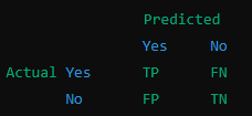
A confusion matrix is a table that helps us understand the performance of a classification model. It compares the actual values with the predicted values and provides insights into the accuracy of the predictions. Here’s how it works:
Structure of a Confusion Matrix
The confusion matrix is typically a 2x2 table for binary classification (where there are only two possible outcomes, like "Yes" or "No"). It looks like this:
Each cell in the table has a specific meaning:
- TP (True Positive): The model predicted "Yes," and the actual value is also "Yes."
- TN (True Negative): The model predicted "No," and the actual value is also "No."
- FP (False Positive): The model predicted "Yes," but the actual value is "No."
- FN (False Negative): The model predicted "No," but the actual value is "Yes."
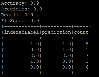
Now you have understand the Confusion Matrix, lets get back to out result of confusion matrix from Iris dataset!
- Class 1.0 (virginica):
- Correctly classified as 1.0 (virginica): 5 instances.
- Incorrectly classified as 0.0 (versicolor): 1 instance.
- Class 0.0 (versicolor):
- Correctly classified as 0.0 (versicolor): 6 instances.
- Incorrectly classified as 1.0 (virginica): 1 instance.
- Class 2.0 (setosa):
- Correctly classified as 2.0 (setosa): 7 instances.
Running the Code Inside Google Colab to have the visualisation
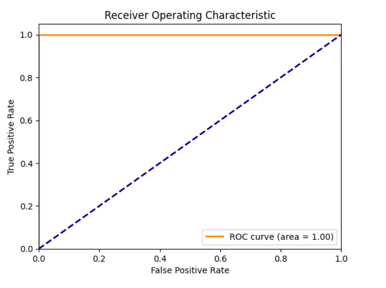
ROC Curve
Insight:
The ROC curve and AUC score of 1.0 confirm that the model is extremely effective in distinguishing between the different classes of the Iris dataset. This high performance is consistent with the confusion matrix results and the metrics of accuracy, precision, recall, and F1-score. Together, they demonstrate that the Random Forest classifier is highly accurate and reliable for this dataset.
The Random Forest classifier performed well on the Iris dataset, achieving high accuracy and balanced precision, recall, and F1-scores.
Specific Results Obtained
-
Accuracy: The model achieved an overall accuracy of 90%, indicating that 90% of the predictions made by the model were correct.
-
Precision: The weighted precision of the model was 90%, indicating the percentage of positive identifications that were actually correct.
-
Recall: The weighted recall of the model was 90%, indicating the percentage of actual positives that were correctly identified.
-
F1-Score: The F1-score was 90%, representing the harmonic mean of precision and recall.
Overall, the model's performance demonstrates its effectiveness in classifying the iris species based on the given features, with high accuracy and balanced evaluation metrics.
💡 Tip: This analysis can be further extended by exploring additional classification algorithms, feature engineering, and further hyperparameter tuning to improve the model's performance.
from pyspark.sql import SparkSession
from pyspark import SparkContext, SparkConf
from pyspark.ml.feature import StringIndexer, VectorAssembler
from pyspark.ml.classification import RandomForestClassifier
from pyspark.ml.evaluation import MulticlassClassificationEvaluator
from pyspark.ml.tuning import CrossValidator, ParamGridBuilder

# Initialize Spark context and session
conf = SparkConf().setAppName("Iris Classification")
sc = SparkContext(conf=conf)
spark = SparkSession(sc)

# Load the Iris dataset
iris_data = spark.read.csv("file:///home/maria_dev/azlin/iris.csv", header=True, inferSchema=True)

# Rename the columns to mathc feature names
iris_data = iris_data.withColumnRenamed("Sepal.Length","sepalLength")\
                     .withColumnRenamed("Sepal.Width","sepalWidth")\
                     .withColumnRenamed("Petal.Length","petalLength")\
                     .withColumnRenamed("Petal.Width","petalWidth")\
                     .withColumnRenamed("Species","label")

# Index labels (convert string labels to numeric)
indexer = StringIndexer(inputCol="label", outputCol="indexedLabel").fit(iris_data)
iris_data = indexer.transform(iris_data)

# Verify the label indexing
label_to_index = {row['label']: row['indexedLabel'] for row in iris_data.select("label", "indexedLabel").distinct().collect()}
print("Label to Index Mapping:", label_to_index)

# Assemble features into a feature vector
assembler = VectorAssembler(inputCols=["sepalLength", "sepalWidth", "petalLength", "petalWidth"], outputCol="features")
iris_data = assembler.transform(iris_data)

# Show the first 5 rows
iris_data.show(5)

# Print
iris_data.printSchema()

# Split the dataset into training and testing sets
train_data, test_data = iris_data.randomSplit([0.8,0.2], seed=42)

# Random Forest is selected as a classification algorithm
randomForest = RandomForestClassifier(labelCol="indexedLabel", featuresCol="features")

#Define a grid of hyperparameter to search over
paramGrid = ParamGridBuilder()\
    .addGrid(randomForest.numTrees, [10,20,30])\
    .addGrid(randomForest.maxDepth, [5,10,15])\
    .build()

# Use cross-validation to tune hyperparameters
crossval = CrossValidator(estimator=randomForest,
                          estimatorParamMaps=paramGrid,
                          evaluator=MulticlassClassificationEvaluator(labelCol="indexedLabel", metricName="accuracy"),
                          numFolds=5)

# Fit the model on the training data
cv_model = crossval.fit(train_data)

# Evaluate the model on the test data
predictions = cv_model.transform(test_data)

# Evaluate the performance of the model
evaluator = MulticlassClassificationEvaluator(labelCol="indexedLabel", predictionCol="prediction")
accuracy = evaluator.evaluate(predictions, {evaluator.metricName: "accuracy"})
precision = evaluator.evaluate(predictions, {evaluator.metricName: "weightedPrecision"})
recall = evaluator.evaluate(predictions, {evaluator.metricName: "weightedRecall"})
f1 = evaluator.evaluate(predictions, {evaluator.metricName: "f1"})

print("Accuracy: {}".format(accuracy))
print("Precision: {}".format(precision))
print("Recall: {}".format(recall))
print("F1-Score: {}".format(f1))

#Collect predictions to a pandas Dataframe for visualisation
predictions.select("indexedLabel", "prediction").groupBy("indexedLabel","prediction").count().show()

sc.stop()


