By Xin Wang, National Institute of Informatics, since 2021
I am a new pytorch user. If you have any suggestions or questions, pleas email wangxin at nii dot ac dot jp
Table of Contents
Updates
2022-01-31: upload project for anti-spoofing confidence estimation
2022-01-08: upload hn-sinc-nsf + hifi-gan
2022-01-08: upload RawNet2 for anti-spoofing
For tutorials on neural vocoders
Tutorials are available in ./tutorials. Please follow the ./tutorials/README and work in this folder first
cd ./tutorials
head -n 2 README.md
# Hands-on materials for neural vocoders
For other projects
Just follow the rest of the README.
The repository is relatively large. You may use --depth 1 option to skip unnecessary files.
git clone --depth 1 https://github.com/nii-yamagishilab/project-NN-Pytorch-scripts.gitThis repository hosts Pytorch codes for the following projects:
-
Harmonic-plus-noise NSF with trainable sinc filter (Hn-sinc-NSF)
-
Hn-sinc-NSF + HiFiGAN discriminator
All the projects include a pre-trained model on CMU-arctic database (4 speakers) and a demo script to run, train, do inference. Please check ./project/01-nsf/README.
Generated samples from pre-trained models are in ./project/01-nsf/*/__pre_trained/output. If not, please run the demo script to produce waveforms using pre-trained models.
Tutorial on NSF models is also available in ./tutorials
Note that this is the re-implementation of the projects based on CURRENNT. All the papers published so far used CURRENNT implementation.
Many samples can be found on NSF homepage.
All the projects include a pre-trained model and a one-click demo script. Please check ./project/05-nn-vocoders/README.
Generated samples from pre-trained models are in ./project/05-nn-vocoders/*/__pre_trained/output.
Tutorial is also available in ./tutorials
It takes time to download ASVspoof2019 database. Therefore, this project demonstrates how to train and evaluate the anti-spoofing model using a toy dataset.
Please try this project before checking other ASVspoof projects below.
A similar project is adopted for ASVspoof2021 LFCC-LCNN baseline, although the LFCC front-end is slightly different.
Please check ./project/04-asvspoof2021-toy/README.
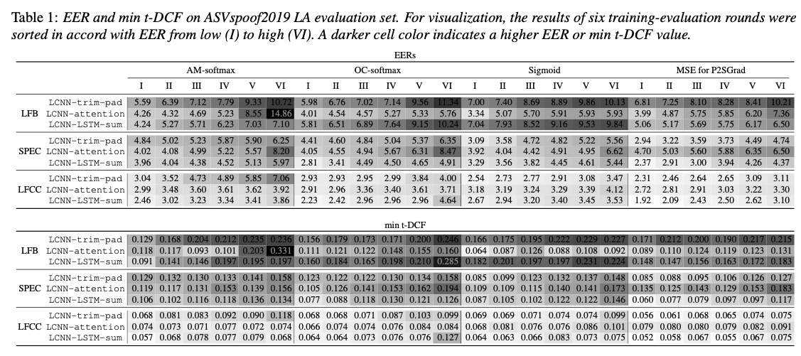
This is for A Comparative Study on Recent Neural Spoofing Countermeasures for Synthetic Speech Detection.
There were 36 systems investigated, each of which was trained and evaluated for 6 rounds with different random seeds.
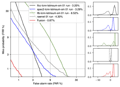
This project is later extended to a book chapter called A Practical Guide to Logical Access Voice Presentation Attack Detection. Single system using RawNet2 is added, and score fusion is added.
Pre-trained models, scores, training recipes are all available. Please check ./project/03-asvspoof-mega/README.
For LCNN, please check this paper; for LFCC, please check this paper; for one-class softmax in ASVspoof, please check this paper.
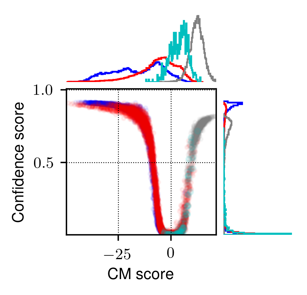
Project for paper https://arxiv.org/abs/2110.04775 (to appear in ICASSP 2022)
Pre-trained models, recipes are all available. Please check ./project/06-asvspoof-ood/README.
You may use ./env.yml to create the environment:
# create environment
conda env create -f env.yml

# load environment (whose name is pytorch-1.6)
conda activate pytorch-1.6Take project/01-nsf/cyc-noise-nsf as an example:
# cd into one project
cd project/01-nsf/cyc-noise-nsf-4

# add PYTHONPATH and activate conda environment
source ../../../env.sh

# run the script
bash 00_demo.sh
The printed info will show what is happening. The script may need 1 day or more to finish.
You may also put the job to the background rather than waiting for the job in front of the terminal:
# run the script in background
bash 00_demo.sh > log_batch 2>&1 &
The above steps will download the CMU-arctic data, run waveform generation using a pre-trained model, and train a new model.
-
Waveform: 16/32-bit PCM or 32-bit float WAV that can be read by scipy.io.wavfile.read
-
Other data: binary, float-32bit, little endian (numpy dtype <f4). The data can be read in python by:
# for a data of shape [N, M]
f = open(filepath,'rb')
datatype = np.dtype(('<f4',(M,)))
data = np.fromfile(f,dtype=datatype)
f.close()
I assume data should be stored in c_continuous format (row-major). There are helper functions in ./core_scripts/data_io/io_tools.py to read and write binary data:
# create a float32 data array
import numpy as np
data = np.asarray(np.random.randn(5, 3), dtype=np.float32)

# write to './temp.bin' and read it as data2
import core_scripts.data_io.io_tools as readwrite
readwrite.f_write_raw_mat(data, './temp.bin')
data2 = readwrite.f_read_raw_mat('./temp.bin', 3)

# result should 0
data - data2
More instructions can be found in the Jupyter notebook ./tutorials/c01_data_format.ipynb.
| Name | Function |
|---|---|
| ./core_scripts | scripts to manage the training process, data io, and so on |
| ./core_modules | finished pytorch modules |
| ./sandbox | new functions and modules to be test |
| ./project | project directories, and each folder correspond to one model for one dataset |
| ./project/*/*/main.py | script to load data and run training and inference |
| ./project/*/*/model.py | model definition based on Pytorch APIs |
| ./project/*/*/config.py | configurations for training/val/test set data |
The motivation is to separate the training and inference process, the model definition, and the data configuration. For example:
-
To define a new model, change model.py
-
To run on a new database, change config.py
The script starts with main.py and calls different function for model training and inference.
During training:

     <main.py>        Entry point and controller of training process
        |
   Argument parse     core_scripts/config_parse/arg_parse.py
   Initialization     core_scripts/startup_config.py
   Choose device
        |
Initialize & load     core_scripts/data_io/customize_dataset.py
training data set
        |----------|
        .     Load data set   <config.py>
        .     configuration
        .          |
        .     Loop over       core_scripts/data_io/customize_dataset.py
        .     data subset
        .          |
        .          |---------|
        .          .    Load one subset   core_scripts/data_io/default_data_io.py
        .          .         |
        .          |---------|
        .          |
        .     Combine subsets
        .     into one set
        .          |
        |----------|
        |
Initialize & load
development data set
        |
Initialize Model     <model.py>
Model(), Loss()
        |
Initialize Optimizer core_scripts/op_manager/op_manager.py
        |
Load checkpoint      --trained-model option to main.py
        |
Start training       core_scripts/nn_manager/nn_manager.py f_train_wrapper()
        |
        |----------|
        .          |
        .     Loop over training data
        .     for one epoch
        .          |
        .          |-------|    core_scripts/nn_manager/nn_manager.py f_run_one_epoch()
        .          |       |
        .          |  Loop over
        .          |  training data
        .          |       |
        .          |       |-------|
        .          |       .    get data_in, data_tar, data_info
        .          |       .    Call data_gen <- Model.forward(...)   <mode.py>
        .          |       .    Call Loss.compute()                   <mode.py>
        .          |       .    loss.backward()
        .          |       .    optimizer.step()
        .          |       .       |
        .          |       |-------|
        .          |       |
        .          |  Save checkpoint
        .          |       |
        .          |  Early stop?
        .          |       | No  \
        .          |       |      \ Yes
        .          |<------|       |
        .                          |
        |--------------------------|
       Done
A detailed flowchat is ./misc/APPENDIX_1.md. This may be useful if you want to hack on the code.
Differences from CURRENNT implementation
There may be more, but here are the important ones:
-
"Batch-normalization": in CURRENNT, "batch-normalization" is conducted along the length sequence, i.e., assuming each frame as one sample;
-
No bias in CNN and FF: due to the 1st point, NSF in this repository uses bias=false for CNN and feedforward layers in neural filter blocks, which can be helpful to make the hidden signals around 0;
-
Smaller learning rate: due to the 1st point, learning rate in this repository is decreased from 0.0003 to a smaller value. Accordingly, more training epochs are required;
-
STFT framing/padding: in CURRENNT, the first frame starts from the 1st step of a signal; in this Pytorch repository (as Librosa), the first frame is centered around the 1st step of a signal, and the frame is padded with 0;
-
STFT backward: in CURRENNT, STFT backward follows the steps in this paper; in Pytorch repository, backward over STFT is done by the Pytorch library.
-
...
The learning curves look similar to the CURRENNT version.

Most of my experiments are done on 16 kHz waveforms. For 24 kHz waveforms, FIR or sinc digital filters in the model may be changed for better performance:
-
hn-nsf: lp_v, lp_u, hp_v, and hp_u are calculated for 16 kHz configurations. For different sampling rate, you may use this online tool http://t-filter.engineerjs.com to get the filter coefficients. In this case, the stop-band for lp_v and lp_u is extended to 12k, while the pass-band for hp_v and hp_u is extended to 12k. The reason is that, no matter what is the sampling rate, the actual formats (in Hz) and spectral of sounds don't change with the sampling rate;
-
hn-sinc-nsf and cyc-noise-nsf: for the similar reason above, the cut-off-frequency value (0, 1) should be adjusted. I will try (hidden_feat * 0.2 + uv * 0.4 + 0.3) * 16 / 24 in model.CondModuleHnSincNSF.get_cut_f();
The end


