Anirban166/atime

atime: Asymptotic Timing

tests
coverage

Installation

## Install last released version from CRAN:
install.packages("atime")

## Install latest version from GitHub:
if(!require("remotes"))install.packages("remotes")
remotes::install_github("tdhock/atime")

Usage

The main function is atime for which you can specify these arguments:

N is numeric vector of data sizes to vary.
setup is an expression to evaluate for every data size, before timings.
times is the number of times each expression is timed (so we can take the median and ignore outliers).
seconds.limit is the max number of seconds. If an expression takes more time, then it will not be timed for larger N values.
there should also be at least one other named argument (an expression to time for every size N, name is the label which will appear on plots).

## When studying asymptotic complexity, always provide sizes on a log
## scale (10^sequence) as below:
(subject.size.vec <- unique(as.integer(10^seq(0,3.5,l=100))))
## Compute asymptotic time and memory measurement:
atime.list <- atime::atime(
  N=subject.size.vec,#vector of sizes.
  setup={#Run for each size, before timings:
    subject <- paste(rep("a", N), collapse="")
    pattern <- paste(rep(c("a?", "a"), each=N), collapse="")
  },
  times=10,#number of timings to compute for each expression.
  seconds.limit=0.1,#max seconds per expression.
  ## Different expressions which will be evaluated for each size N:
  PCRE.match=regexpr(pattern, subject, perl=TRUE),
  TRE.match=regexpr(pattern, subject, perl=FALSE),
  constant.replacement=gsub("a","constant size replacement",subject),
  linear.replacement=gsub("a",subject,subject))
atime.list
plot(atime.list)
## Compute and plot asymptotic reference lines:
(best.list <- atime::references_best(atime.list))
plot(best.list)
## Compute and plot data size N for given time/memory.
pred.list <- predict(best.list, seconds=1e-2, kilobytes=10)
plot(pred.list)

Time/memory comparison overview

On my machine I got the following results:

> (subject.size.vec <- unique(as.integer(10^seq(0,3.5,l=100))))
 [1]    1    2    3    4    5    6    7    8    9   10   11   12   13   14   15
[16]   17   18   20   22   23   25   28   30   33   35   38   42   45   49   53
[31]   58   63   68   74   81   87   95  103  112  121  132  143  155  168  183
[46]  198  215  233  253  275  298  323  351  380  413  448  486  527  572  620
[61]  673  730  792  859  932 1011 1097 1190 1291 1401 1519 1648 1788 1940 2104
[76] 2283 2477 2687 2915 3162

The vector above is the sequence of sizes N, used with each expression, to measure time and memory. When studying asymptotic complexity, always provide sizes on a log scale as above.

> atime.list
atime list with 228 measurements for
PCRE.match(N=1 to 20)
TRE.match(N=1 to 275)
constant.replacement(N=1 to 3162)
linear.replacement(N=1 to 3162)

The output above shows the min and max N values that were run for each of the expressions. In this case constant.replacement and linear.replacement were run all the way up to the max size (3162), but TRE.match only went up to 20, and PCRE.match only went up to 275, because no larger N values are considered after the median time for a given N has has exceeded seconds.limit which is 0.1 above. This behavior ensures that total time taken by atime will be about seconds.limit * times * number of expressions (times is the number of times each expression is evaluated at each data size). 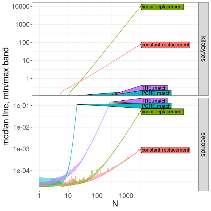The output of the plot method for this atime result list is shown below,

> plot(atime.list)

The plot above facilitates comparing the time and memory of the different expressions, and makes it easy to see the ranking of different algorithms, but it does not show the asymptotic complexity class.

Asymptotic complexity class estimation

To estimate the asymptotic complexity class, use the code below:

> (best.list <- atime::references_best(atime.list))
references_best list with 456 measurements, best fit complexity:
constant.replacement (N kilobytes, N seconds)
linear.replacement (N^2 kilobytes, N^2 seconds)
PCRE.match (2^N seconds)
TRE.match (N^3 seconds)

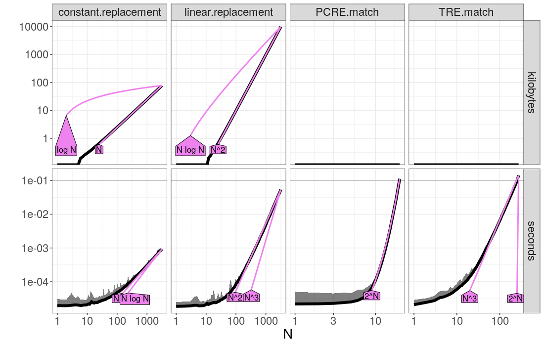
The output above shows the best fit asymptotic time complexity for each expression. To visualize the results you can do:

plot(best.list)

The plot above shows the timings of each expression as a function of data size N (black), as well as the two closest asymptotic reference lines (violet, one smaller, one larger). If you have chosen N and seconds.limit appropriately for your problem (as we have in this case) then you should be able to observe the following:

on the left you can see timings for small N, where overhead dominates the timings, and the curve is approximately constant.
on the right you can see the asymptotic trend.
- Polynomial complexity algorithms show up as linear trends, and the slope indicates the asymptotic complexity class (larger slope for more complex algorithm in N).
- Exponential complexity algorithms show up as super-linear curves (such as PCRE.match in this case, but in practice you should rarely encounter exponential time algorithms).
If you do not see an interpretable result with clear linear trends on the right of the log-log plot, you should try to increase seconds.limit and the max value in N until you start to see linear trends, and clearly overlapping reference lines (as is the case here).

Highlight N for given time/memory

When comparing algorithms in terms of computational resources, we can either

show the time/memory required for a given data size N, or
show the data size N possible for a given time/memory budget.

We can do both using the code below,

> atime.list[["measurements"]][N==323, .(expr.name, seconds=median, kilobytes)]
              expr.name   seconds kilobytes
                 <char>     <num>     <num>
1:            TRE.match 0.0678032    0.0000
2: constant.replacement 0.0000667    7.9375
3:   linear.replacement 0.0002435  101.9375
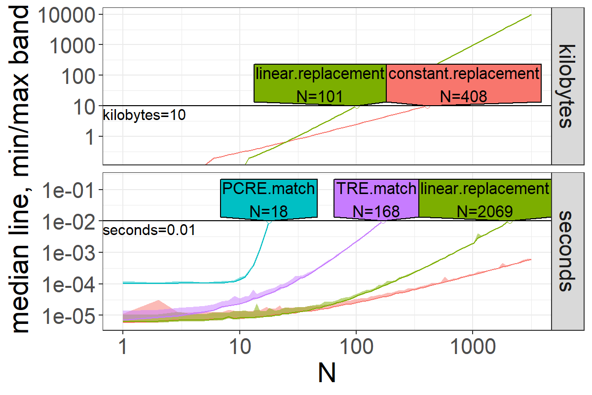
> pred.list <- predict(best.list, seconds=1e-2, kilobytes=10)
> pred.list[["prediction"]]
        unit            expr.name unit.value          N
      <char>               <char>      <num>      <num>
1:   seconds           PCRE.match       0.01   17.82348
2:   seconds            TRE.match       0.01  168.46338
3:   seconds   linear.replacement       0.01 2069.38604
4: kilobytes constant.replacement      10.00  407.55220
5: kilobytes   linear.replacement      10.00  100.92007
> plot(pred.list)

Related work

bench::press does something similar, and is more flexible because it can do multi-dimensional grid search (not only over a single size N argument as atime does). However it can not store results if check=FALSE, results must be equal if check=TRUE, and there is no way to easily specify a time limit which stops for larger sizes (like seconds.limit argument in atime).

testComplexity::asymptoticTimings does something similar, but only for one expression (not several), and there is no special setup argument like atime (which means that the timing must include data setup code which may be irrelevant).

Anirban166 / atime