This project is part of the Udacity Azure ML Nanodegree. In this project, we build and optimize an Azure ML pipeline using the Python SDK and a provided Scikit-learn model. This model is then compared to an Azure AutoML run.
The primary objective of this model development and deployment is to build a method for predicting the marketing overturn for different clients by correlating the prediction to contextual inputs such as profession, job, marital status, education, period, duration, campaign information and so on. The main metric to predict is the possibilit of the individual returning a positive reaction or replying back to a marketing campaign by the bank. As a result, the ouput is of a dichotomous nature where it represents two possible outcomes- a yes or a no. Based on the predictive models that were used in this study, we can conclude that VotingEnsemble is the best method for predicting the outputs and offers the highest accuracy, which is only slightly better than the HyperdriveCongig paramterization.
The pipeline architecture consists of a computing instance cluster and inference cluster where the models are stored. The preprocessing data transformation steps are executed using the Explain the pipeline architecture, including data, hyperparameter tuning, and classification algorithm.
The parameter sampler used for this project is well suited for dichotomous outputs, especially for models that require logistic regression based paramterization to achieve the best results in terms of accuracies. It spans out the best possible combinations of maximum iterations and loss functions(represented by the --C regularization parameter). What are the benefits of the parameter sampler you chose? The classification algorithm used is for logistic regression and checks for various choices of both maximum iterations and --C inputs. The primary metric has been set to accuracy and the primary metric goal is to maximize this accuracy. The alternative to this is the use of the Loss function which requires more time and is beyond the scope of the project. The main advantage of using the Random Sampler is the fact that each data point has an equal probability of being selected which may not be possible with alternatives like grid sampling which chooses input points at predetermined intervals. Random Samplers can be difficult to execute because of this equal partitioning but are safe from skewed predition results which can plague other types of samplers. Random Sampling confugrations are also simple enough to be maniuplated by changing metrics like number of concurrent runs and cut off percentages. In the context of this project. The smaller number of sampling metrics to choose from and the balanced nature of the dataset(nearly equal portions of yes and no outputs), makes grid sampling cumbersome and time consuming. What are the benefits of the early stopping policy you chose? The early stopping policy selected for this project, as per the instructions, is the Bandit Policy which stresses on the use of slack amounts and intervals such that the run is terminated if the primary metric is not within the threshold of the best run. This saves time and also helps in narrowing down the best algorithms that can perform faster predictions to the rest.
In 1-2 sentences, describe the model and hyperparameters generated by AutoML.
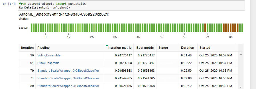
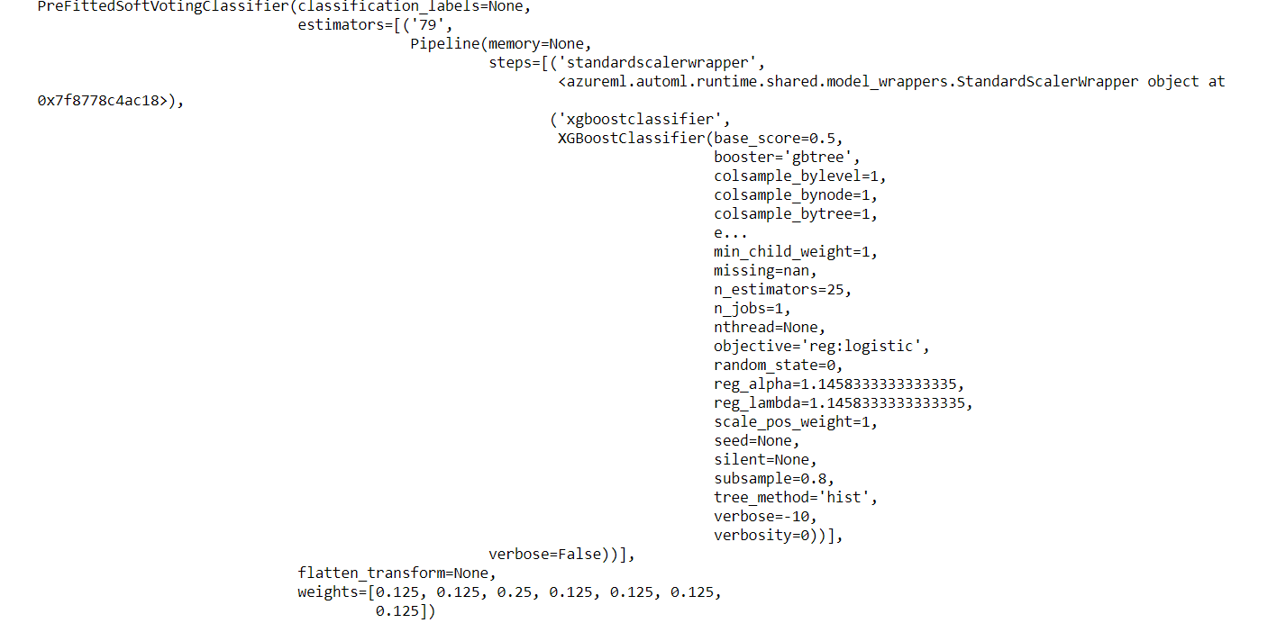
Tge AutoML algorithm, as the name applies, takes in the best parameters specified by the user for the training and testing distribution along with the cross validation score, the tasks, number of iterations and primary metric. AutoML uses these metrics to span through its existing repository of algorithms and performs the same level of abstracted analysis to obtain the best models. To ensure that the AutoML run doesn't go on interminably, the user adds a stopping factor or an experimental timeout metric. As seen in the image below, we can see the results of the AutoML runs using the y metric as the predictor from the dataset provided.
Compare the two models and their performance. What are the differences in accuracy? In architecture? If there was a difference, why do you think there was one?


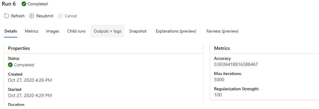
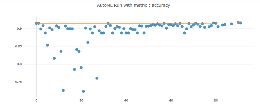
With repeated runs, it can be ascertained that the accuracies for both the hyperdrive algorithm and the AutoML algorithm are similar in terms of accuracies(a 90% achieved with the hyperdrive while ~91% using the AutoML generator). It should be noted that the accuracies obtained from AutoML are more suitable as the system arrives at the best configuration for the algorithm. The MaxAbsScaler LightGBM algorithm returned the best accuracy with a 0.9148 output. The hyperparameters for the best AutoML generated model are 79 estimators, base score=0.5, booster='gbtree', colsample_bylevel=1, colsample_bynode=1, colsample_bytree=1, min_child_weight=1, reg_alpha=1.1458333333333335, reg_lambda=1.1458333333333335, tree_method='hist', C=1.0, class_weight=None, max_iter=100, multi_class='auto', n_jobs=None, penalty='l2', solver='lbfgs', tol=0.0001.
Both architectures can be seen and compared in the images below.

The difference is definitely a result of the difference in the batch size of the runs and the maximum number of iterations performed. A bigger difference can also be linked to the use of different algorithms in both cases.


What are some areas of improvement for future experiments? Why might these improvements help the model? For future experiments, the project can be expanded to include other metrics for logistic regression studies such as maximum number of batch sizes, loss functions, L2 regularization and median absolute errors. Classification reports from the XGBoosting function can be expanded to include a matrix for false positives, false negatives, true positives and true negatives. The threshold for parameters can also be expanded to include a wider range. All these steps will help in providing a clearer interpretation of the models and their approach to predicting the output.
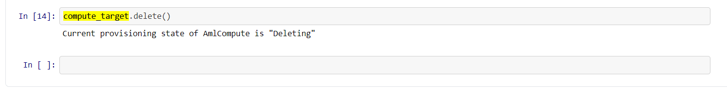
The proof for the deletion of the compute cluster can be seen from the image below. The same can be confirmed through the Hyperdrive.ipynb file on the repository.