AliMorty / Big_Data_Project

Exploring the paper titled: Learning Mixture of Gaussians with Streaming Data, NIPS17

Big Data Project

Learning Mixture of Gaussians with Streaming Data

This project is done by me, aminrashidbeigi and Bita Jalali.

1. Abstract

In this project, we explore a theoretical paper published in Neurips2017 Conference titled Learning Mixture of Gaussians with Streaming Data by doing some experimental tests on the performance of the algorithm. You can find the original paper here.
The authors of the paper proposed an algorithm with a theoretical guarantee for the problem of clustering the streaming data points where data points come from a Mixture of Gaussian Distribution. In particular, they showed that with high probability, the algorithm eventually finds (/learns) the mixture of Gaussians accurately. Moreover, they showed that the learning rate is near-optimal. Meaning that in each step, the error decreases optimally. Note that, as the problem of learning the mixture of Gaussian is NP-Hard, they used a simplification assumption for the data to make the problem tractable. The simplification assumption they used is that data comes from a mixture of well-separated Gaussians. (i.e. the centers of any two clusters are far enough so that the algorithm can decide computationally easily whether the point belongs to the first cluster or the second one.)
Although the assumption allows them to have a good performance for this problem, one question might arise: Is the analysis of the paper tight?
One way to find an answer to this question is to test the algorithm's performance by running some experimental tests. Of course, the experimental tests just provide evidence and they are not proof.

You can find the report in the HTML format. (In case you can't read the formulas here.)

2. Project Outline

In the following, we will first give a bit explanation about the general setup and data distribution in the first section. Then we explain the theorems about the performance of the algorithm. Finally, we test the algorithm performance by generating data from the mixture of Gaussian Distribution and run our implementation of the paper's algorithm

3. Setup

3.1. Data Distribution

Data is drawn from a mixture of a mixture of k spherical Gaussians distributions,
i.e. for all $i = 1,2,...,k$: $$ x^t {\sim} \sum_{i} w_i \mathcal{N}(\mu_i^, \sigma^2 I) , \sigma_i^ \in \mathcal{R}^d $$

where $\mu_i^*$ is the mean of the i-th mixture component (i-th cluster), mixture weights $w_i \geq 0$, and $\sum_i wi = 1$.
For simplicity, we assumed all $\sigma_i=\sigma$ are the same. But the algorithm doesn't require this assumption.

3.2. Seperation Assumption

As we stated earlier, the paper used a simplification assumption for the data. In particular, any two centers $i , j$ should be far away from each other at least $C \sigma $ i.e.: $$ ||\mu_i^* - \mu_j^*|| \geq C \sigma $$

We will explain more about the constant C in the next sections.

3.3 Space Overview

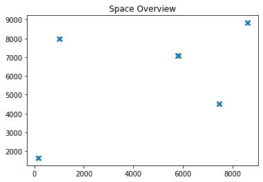
100 points drawn from the distribution are depicted here. (note that we have shown a 2-d subspace from the original d-dimensional space of data points.
You can see there are k clusters.

temp = generator.generate_samples(100)
plt.plot(temp[0, :], temp[1,:], 'x')
plt.title("Space Overview")
plt.show()

4. Algorithm Overview

The algorithm consists of two parts:
1 . Algorithm1 (initialization algorithm)
2 . Algorithm2: (a) Streaming using Lloyd's Heuristic, (b) Expectation Maximization (i.e.Soft version of Lloyd's Heuristic)

Note that Expectation Maximization part is available in another file named "EM".

4.1 Initialization Algorithm

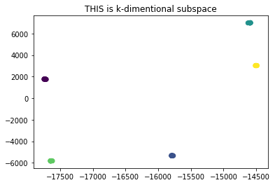
In the initialization part, we try to find k initial centers for k clusters. To do so, we first use SVD-style operations to project d dimensional data points into a k-dimensional space. These operations project will de-noise the data, making it easy for the algorithm to identify all k distinct clusters from few data points. After we find k clusters centers in the projected space, we project them to the original d-dimensional space. This way, we have a good initialization for the k centers.

import numpy as np
import matplotlib.pyplot as plt
from scipy.stats import ortho_group
from scipy import linalg
import random
from sklearn import neighbors
import sklearn.metrics.pairwise
from scipy.sparse import csgraph
import random
import pandas as pd


d = 10
k = 5
scaler = 10000
sigma = 100
num_of_samples = int(d*d*d*k*k*k*np.log(d*k))  #N0
w = np.ones(k) / k

## For initializatoin, we need C to be at least OMEGA((klogk)^1/4). So:
C = 10*((k*np.log(k))**(1/4))
C2 = (np.log(k)**(1/2))
##TODO: Change max to min but make sure that you ignore the diagonal values as they are zeros and they should be ignored. 
def generate_distant_means(dimension, C, std):
    mu = np.random.rand(d, k) * scaler
    dist = sklearn.metrics.pairwise.euclidean_distances(mu.T)
    dist = dist + np.identity(k, dtype = float) * 2 * C * sigma
    min_dist = np.min(dist)
    while (min_dist < C * sigma):
        print ("close_initial_points_occured, start again")
        mu = np.random.rand(d, k) * scaler
        dist = sklearn.metrics.pairwise.euclidean_distances(mu.T)
        dist = dist + np.identity(k, dtype = float)   * 2 * C * sigma
        min_dist = np.min(dist)
    return mu

mu = generate_distant_means(d, C, sigma)
print ("True Centers for Clusters")

tmp = pd.DataFrame(mu)
tmp

True Centers for Clusters

<style scoped> .dataframe tbody tr th:only-of-type { vertical-align: middle; }

.dataframe tbody tr th {
    vertical-align: top;
}

.dataframe thead th {
    text-align: right;
}

</style>

	0	1	2	3	4
0	1006.573560	7457.903141	8607.361205	5805.062752	159.473022
1	7981.089236	4519.639663	8843.143067	7082.612751	1638.453342
2	1786.589980	7512.222316	4686.177980	1062.615207	6604.511910
3	3298.659779	8089.362560	6149.617684	4718.901034	7559.245778
4	8864.726130	5712.461236	1803.188495	7849.071028	7154.246706
5	7637.138501	6373.934348	3263.415539	1354.105588	2977.484326
6	6208.651794	2407.470493	1071.618747	5643.999592	3806.159423
7	2173.689721	828.673876	1893.492336	2113.814978	2271.450202
8	5882.354979	1509.902750	6242.963681	8404.339237	9478.986709
9	9055.694116	9003.731212	6530.270935	1714.366744	2276.888733

Sample Generator Class

class SampleGenerator:
    def __init__(self, weights, mu, sigma, d):
        self.weights = weights
        self.mu = mu
        self.sigma=sigma
        self.d = d
    
    def draw_a_sample(self):
        rand = random.uniform(0,1)
        for i in range(len(self.weights)):
            rand -= self.weights[i]
            if (rand <=0):
                return np.random.multivariate_normal(self.mu[:,i], self.sigma * np.identity(self.d), 1).T
    
    def generate_samples(self, sample_size):
        samples = []
        for i in range(sample_size):
            if len(samples) == 0:
                samples = self.draw_a_sample()
            else:
                samples = np.append(samples, self.draw_a_sample(), axis=1)
        return samples

generator = SampleGenerator(w, mu, sigma, d)

4.1.1 Finding k-dimensional subspace using Streaming PCA method

In this part, we are going to find a k dimensional space to reduce the noise of each cluster. This way, all points from a single clusters will become closer to each other, allowing us to use Nearest Neighbor Graph to identify each cluster easily.

N0 = num_of_samples

S = np.zeros((d, d))
k_2 = int(10 * k * np.log(k))
B = int(d * np.log(d))
U = ortho_group.rvs(dim=d)[:, :k]  # Choosing k orthonormal vectors in Rd space

for t in range(N0 - k_2):
    if t % B == B - 1:
        Q, R = linalg.qr(np.matmul(S, U))
        U = Q
        S = np.zeros((d, d))
    reshaped_sample = generator.draw_a_sample().reshape(-1, 1)
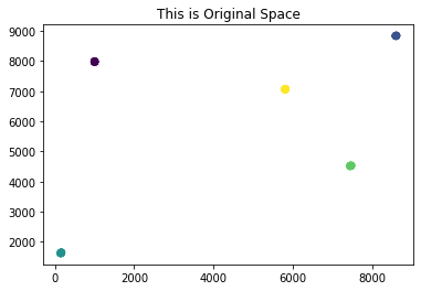
    S = S + np.matmul(reshaped_sample, reshaped_sample.T)

4.1.2 Using Nearest Neighbor to find all k clusters

First, we project points to the k-dimensional space to reduce the noise, then using each point as a node, we build a nearest neighbor graph. Each connected component in the graph would represent a cluster.

X0 = generator.generate_samples(k_2)
save_U = U
U = U[:, 0:k]
components = np.matmul(U.T, X0)
adj = neighbors.kneighbors_graph(np.transpose(components), 3)
n_components, labels = csgraph.connected_components(adj)

fig, ax = plt.subplots()
ax.scatter(components[0], components[1], c=labels)
plt.title("THIS is k-dimentional subspace")
plt.show()

components = np.matmul(U, components)
fig, ax = plt.subplots()
ax.scatter(components[0], components[1], c=labels)
plt.title("This is Original Space")
plt.show()

components_mean = np.zeros((k, d))
components_by_labels = []
for c in range(k):
    list_of_indices = np.where(labels == c)[0]
    components_mean[c] = np.mean(components[:, list_of_indices], axis=1)
    
print("Components mean:")
pd.DataFrame(components_mean.T)

Components mean:

<style scoped> .dataframe tbody tr th:only-of-type { vertical-align: middle; }

.dataframe tbody tr th {
    vertical-align: top;
}

.dataframe thead th {
    text-align: right;
}

</style>

	0	1	2	3	4
0	1004.659735	8602.688447	156.998482	7457.114878	5810.833626
1	7981.449254	8842.145440	1632.891263	4523.029546	7070.616973
2	1790.712167	4682.362683	6602.861160	7512.045539	1061.278888
3	3296.125969	6153.697604	7558.724763	8092.409179	4712.346784
4	8863.349343	1806.231879	7152.189040	5715.178904	7845.894733
5	7628.245490	3258.963132	2980.991991	6375.568134	1361.207542
6	6215.085481	1067.861391	3807.590765	2404.595059	5642.911509
7	2169.924317	1889.896869	2275.113901	832.385092	2119.977969
8	5885.804747	6239.186480	9477.207032	1509.366177	8414.359976
9	9054.406525	6531.609386	2277.226207	9008.111500	1717.347722

print ("TRUE centers")
pd.DataFrame(mu)

TRUE centers

<style scoped> .dataframe tbody tr th:only-of-type { vertical-align: middle; }

.dataframe tbody tr th {
    vertical-align: top;
}

.dataframe thead th {
    text-align: right;
}

</style>

	0	1	2	3	4
0	1006.573560	7457.903141	8607.361205	5805.062752	159.473022
1	7981.089236	4519.639663	8843.143067	7082.612751	1638.453342
2	1786.589980	7512.222316	4686.177980	1062.615207	6604.511910
3	3298.659779	8089.362560	6149.617684	4718.901034	7559.245778
4	8864.726130	5712.461236	1803.188495	7849.071028	7154.246706
5	7637.138501	6373.934348	3263.415539	1354.105588	2977.484326
6	6208.651794	2407.470493	1071.618747	5643.999592	3806.159423
7	2173.689721	828.673876	1893.492336	2113.814978	2271.450202
8	5882.354979	1509.902750	6242.963681	8404.339237	9478.986709
9	9055.694116	9003.731212	6530.270935	1714.366744	2276.888733

4.1.3 Thoerem 3

As we know in the Theorem 3 of the paper, if each two centers have enough seperations, $\Omega (k \log k )^{1/4}$,
then with high probability $1 - \dfrac{1}{poly(k)}$, the distance between TRUE center and algorithm's output can be bounded by
$$|| \mu_i^0 - \mu_i^*|| \leq \dfrac{C}{20}\sigma$$

4.1.4 Verifying Theorem 3: Comparision Between "Alg centers output" and "TRUE centeres"

def distance_calculator(mu, mu_t):
    comparision_matrix = sklearn.metrics.pairwise.euclidean_distances(mu.T, mu_t.T)
    distance_vector = np.min(comparision_matrix, axis=0)
    distance_sum = np.sum(np.min(comparision_matrix, axis=0))

    return distance_sum, distance_vector

distance_sum, distance_vector = distance_calculator(mu, components_mean.T)

DF = pd.DataFrame(distance_vector)
DF.columns = ["Distance"]
print ("Distance between each cluster center and algorithm's output for that center:")
print(DF)

print("Sum of distances:")
print(distance_sum)

Distance between each cluster center and algorithm's output for that center:
    Distance
0  13.315987
1  11.234860
2   8.680253
3   8.543820
4  20.759095
Sum of distances:
62.53401504530203

theorem3_bound= C*sigma/20

print ("Theorem 3 Bound: C/20 * sigma")
theorem3_bound

Theorem 3 Bound: C/20 * sigma





8.421337295817725

As you can see, the TRUE MEANS are very close to initial algorithm's output as desired.

4.2 Streaming Clustering (using Lloyd Heuristic)

In this part, we are going to use the Lloyd Heuristic for clustering. Uppon the arrival of each data point, we firstly assign it to its closest center and then update that center.

from numpy import linalg as LA
import copy

mu01 = components_mean.T


def streaming_kmeans(n, input_mu, num_of_logs):
    mu0 = copy.deepcopy(input_mu)
    distance_log = []
    eta = 3 * k * (np.log2(3 * n)) / n
    cut = int(n / num_of_logs)
    for t in range(n):
        if t % cut == 0:
            d, _ = distance_calculator(mu, mu0)
            distance_log.append(d)
        x = generator.draw_a_sample()

        dis = LA.norm((x - mu0), axis=0)
        i = np.argmin(dis)
        x = x.reshape(-1)
        mu0[:, i] = np.multiply((1 - eta), mu0[:, i]) + np.multiply(eta, x)
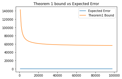
    return mu0, distance_log

4.2.1 Theroem 1

Intuitively, this theorem upper bounds the error when we have seen enough data.

Let $xt, 1 \leq t \leq N + N_0$ be generated using a mixture of Gaussians with wi = 1/k, for all i, Let $N_0, N \geq O(1)k^3d^3 \log d $ and $ C \geq \Omega {(k\log k)^{1/4}}$. Then, the algorithm's output satifies the following error bound:

$$ \mathbb{E}(|| \mu^0 - \mu^* ||^2 ) \leq \dfrac{\max_i ||\mu_i^* ||^2 }{N^{\Omega(1)}} + O(k^3)(\sigma^2\dfrac{d\log N}{N} + \exp (-C^2/8)(c^2+k)\sigma^2) $$

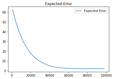
In the following, we will verify theorem 1 experimentally.

def theorem_1(mu, N, sigma, K, C, d):
    return (np.max(LA.norm(mu,axis=0)) / N) + (K**3 * (sigma**2 * d * np.log(N) / N) + np.exp(-C**2 / 8) * (C**2 + K)* sigma**2)

num_of_logs = 1000

run_count = 10
error_matrix = np.zeros((run_count, num_of_logs))
Ns = []
n = 2*int(d*d*d*k*k*k*np.log(d*k))
for run in range(run_count):
    mu_t, distance_log = streaming_kmeans(n, mu01, num_of_logs)
    error_matrix[run] = distance_log[:num_of_logs]
df=pd.DataFrame(error_matrix)

mean_error = np.mean(error_matrix, axis=0)
diagram_cut = 100

theorem_1_log = []
Ns = []
for i in range(num_of_logs):
    cut = int(n / num_of_logs)
    theorem_1_log.append(theorem_1(mu, cut * (i+1), sigma, k, C, d))
    Ns.append(cut * (i+1))
    
p1, =plt.plot(Ns[:diagram_cut], mean_error[:diagram_cut], label='Expected Error')
plt.legend(loc='best')
plt.title('Expected Error')
plt.show()

p1, =plt.plot(Ns[:diagram_cut], mean_error[:diagram_cut], label='Expected Error')
p2, =plt.plot(Ns[:diagram_cut], theorem_1_log[:diagram_cut], label='Theorem1 Bound')
plt.legend(loc='best')
plt.title('Theorem 1 bound vs Expected Error')
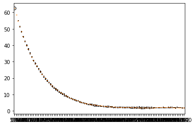
plt.show()

boxplot_dict = {}

for i in range(diagram_cut):
    boxplot_dict[cut * (i+1)] = [np.mean(error_matrix[:, i]), np.min(error_matrix[:, i]), np.max(error_matrix[:, i]), ]

fig, ax = plt.subplots()
ax.boxplot(boxplot_dict.values())
ax.set_xticklabels(boxplot_dict.keys())
plt.plot()

[]

4.2.2 Theorem 2

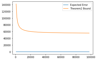
The streaming part of the algorithm works even when the data seperation C is much less. (when $ C \geq \Omega (\log k)^{1/2} $)
In this part, we will verify it experimentally in the following cell.

theorem_2_log = []
for i in range(num_of_logs):
    cut = int(n / num_of_logs)
    theorem_2_log.append(theorem_1(mu, cut * (i+1), sigma, k, C2, d))
    
p1, =plt.plot(Ns[:diagram_cut], mean_error[:diagram_cut], label='Expected Error')
p2, =plt.plot(Ns[:diagram_cut], theorem_2_log[:diagram_cut], label='Theorem2 Bound')
plt.legend(loc='best')
plt.show()