WD_models

(Updated on Feb 22, 2021. For details of updates please check update.md)

The number of white dwarfs (WD) with precise luminosity and color measurements has been increased drastically by Gaia DR2. Accordingly, the need for a tool to easily transform WD photometry to physical parameters (and vice versa) emerges. Here, I provide a python package for such transformations, based on interpolation of existing WD atmosphere grid and cooling models. This package is written for python 3 and depends on the following packages: astropy, numpy, scipy. The most useful functions include:

converting the coordinates of Gaia (and other passbands) H--R diagram into WD parameters;
plotting contours of WD parameters on the Gaia (and other passbands) H--R diagram.

It also provides tools to transform any desired WD parameters and compare the results of different WD models. In addition, the user may custimize many parameters, such as the choice of cooling models and setting details of plotting.

If you use this tool, don't forget to cite this website and the corresponding papers of synthetic colors and cooling models (see the reference at the bottom of this page). If you have more cooling models and/or synthetic colors, I am more than happy to add them to this package!

Below, I introduce the basic usage of this package, give some examples. A list of available cooling models is attached. I also present a detailed introduction to the output of the main function load_model. I hope that with a convenient way provided to transform WD parameters, more researchers will be attracted to the WD field, and the connection between observers, theorists, and astronomers from outside the WD field will be tighter. For questions or suggestions or comments, please do not hesitate to contact me: s.cheng@jhu.edu

Install

Just download the package WD_models to some local path in your computer. If that path is not included in python's system's path, then you need to add it. For example, if you download the WD_models package (which is a folder) to '~/softwares/', then the following codes should import the package smoothly.

import sys
sys.path.append('~/softwares/')
import WD_models

Example 1: converting H--R diagram coordinate into WD parameters

model = WD_models.load_model(low_mass_model='Bedard2020',
                             middle_mass_model='Bedard2020',
                             high_mass_model='ONe',
                             atm_type='H',
                             HR_bands=('bp3-rp3', 'G3'))
bp3_rp3 = np.array([0.25, 0.25])
G3 = np.array([13,14])
age_cool = model['HR_to_age_cool'](bp3_rp3, G3)

print('bp3_rp3: ', bp3_rp3, '\nM_G3: ', G3)
print('cooling ages:', age_cool, 'Gyr')
>> bp_rp:	[ 0.25  0.25] 
>> M_G:	[13 14]
>> cooling ages: [ 1.31350174  2.74414148] Gyr

The outputs are in unit of Gyr. The function load_model in the package reads a set of cooling tracks and returns a dictionary containing many useful functions for parameter transformation and grid data for ploting contours. The keys of this dictionary are listed in the section "output of the function load_model" below.

With the argument HR_bands, one can change the passband for both the color index and absolute magnitude of the H--R diagram. It can be any combination from the following bands:

filter system	filters	filter names in this package
Gaia EDR3	G, bp, rp	G3, bp3, rp3
Gaia DR2	G, bp, rp	G2, bp2, rp2
SDSS	u, g, r, i, z	Su, Sg, Sr, Si, Sz
PanSTARRS	g, r, i, z, y	Pg, Pr, Pi, Pz, Py
Johnson	U, B, V, R, I	U, B, V, R, I
2MASS	J, H, Ks	J, H, Ks
Mauna Kea Observatory (MKO)	Y, J, H, K	MY, MJ, MH, MK
WISE	W1, W2, W3, W4	W1, W2, W3, W4
Spitzer	3.6, 4.5, 5.8, 8.0	S36, S45, S58, S80
GALEX	FUV, NUV	FUV, NUV

For example:

model = WD_models.load_model('be', 'be', 'o', 'H',
                             HR_bands=('Su-Sg', 'G3'),)

Note that shorter names of the same cooling models (see section "Available models included in this package" below for details) are used here.

Loading two sets of models allows comparisons between cooling models. For example:

model_A = WD_models.load_model('', 'be', 'be', 'H')
model_B = WD_models.load_model('', 'be', 'be', 'He')

d_age_cool = (model_A['HR_to_age_cool'](0, 13) - model_B['HR_to_age_cool'](0, 13))

print('bp3-rp3 = 0,  M_G3 = 13')
print('difference of cooling ages between DA and DB models: ', d_age_cool, 'Gyr')
>> bp3-rp3 = 0,  M_G3 = 13
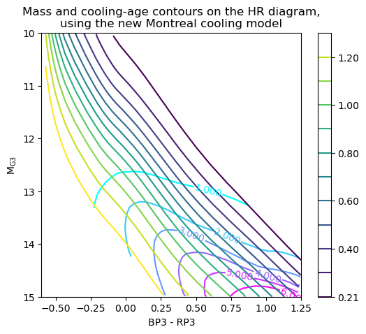
>> difference of cooling ages between DA and DB models:  0.1695180723420473 Gyr

Example 2: plotting contours on the H--R diagram

The contours can be plotted using the grid data in the output of function load_model. To make sure the coordinates match, the argument HR_grid of function load_model should be used, and the same values should also be used for the extent of contour plotting.

HR_grid = (-0.6, 1.25, 0.002, 10, 15, 0.01)
model = WD_models.load_model('be', 'be', 'be', 'H', HR_grid=HR_grid)
extent = (HR_grid[0], HR_grid[1], HR_grid[3], HR_grid[4])
plt.contour(model['grid_HR_to_mass'].T, extent=extent)
plt.contour(model['grid_HR_to_age_cool'].T, extent=extent)

Codes for plotting the exact figure (and figures below) are provided in the jupyter notebook /WD_models_examples.ipynb.

A comment: The total age is a very steep function of white dwarf mass and not suitable for interpolation. So, for plotting the contour or other use of the total age, the following way is recommend:

plt.contour(
    model['grid_HR_to_age_cool'].T + WD_models.MS_age(model['grid_HR_to_mass'].T)*1e-9,
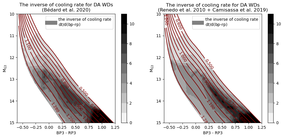
    extent=extent)

Example 3: the effect of phase separation

In the output of function load_model I also provide the cooling rate information dt / d(bp-rp), which is the inverse of cooling rate. If the cooling is low in one region of the H--R diagram, WDs will pile-up there; the number density on the H--R diagram is proportional to the inverse of cooling rate dt / d(bp-rp). The above figures are the inverse of cooling rate for two different models.

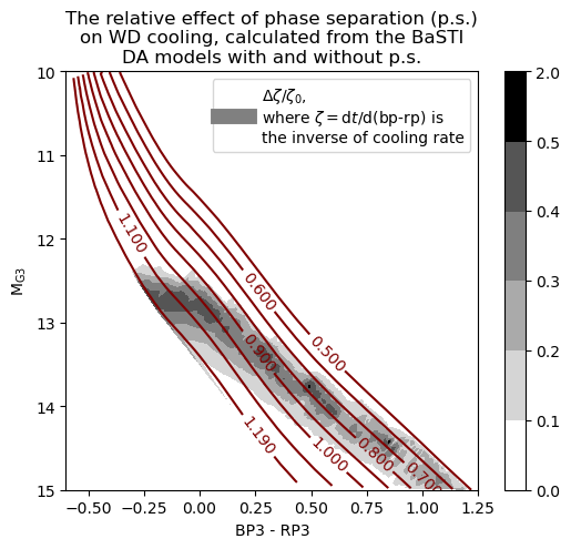
plt.contourf(model['grid_HR_to_cool_rate^-1'].T, extent=extent)

I also show an interesting visualization based on the BaSTI cooing tracks with and without phase separation.

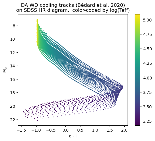
Example 4: plotting cooling tracks on H--R diagram

For DA white dwarfs, there is a turning of color at low temperature. So, when interpolating the mapping HR --> WD parameters, I cut off the low-temperature part to avoid artifacts. This cut can be set with the argument logteff_logg_grid, which includes six elements for (xmin, xmax, dx, ymin, ymax, dy), and the default value for min_logteff is 3.5, i.e. Teff about 3200 K.

For ploting the cooling-tracks data points on the H--R diagram, the low-temperature cut is not necessary. So, the first element in logteff_logg_grid can be set to a lower value to avoid this cut:

logteff_logg_grid = (3.0, 5.1, 0.01, 6.5, 9.6, 0.01)
model = WD_models.load_model('be', 'be', 'be', 'H', 
                             HR_bands=('Sg-Si','Sg'), 
                             logteff_logg_grid=logteff_logg_grid)
plt.scatter(model['color'], model['Mag'], c=model['logteff'])

Note that this H--R diagram is for SDSS passbands.

Example 5: transformation between any desired WD parameters

If a desired transformation function is not provided in the output of load_model, e.g., (mass, Teff) --> cooling age, the user can generate the customized mapping with the functions interp_xy_z_func, interp_xy_z, or interp_HR_to_para provided in this package. These functions read the cooling-track data points from the output of load_model and then generate new mappings.

For example, for the mapping (mass, logteff) --> cooling age:

model = WD_models.load_model('be', 'be', 'o', 'H')

# interpolate the desired mapping
m_logteff_to_agecool = WD_models.interp_xy_z_func(x=model['mass_array'],
                                                  y=model['logteff'],
                                                  z=model['age_cool'],
                                                  interp_type='linear')
                                                  
# calculate the cooling age for (m_WD, Teff) = (1.1 Msun, 10000 K)
age_cool = m_logteff_to_agecool(1.1, np.log10(10000))

print('mass: 1.1 Msun,  Teff: 10000 K')
print('cooling age: ', age_cool, 'Gyr')
>> mass: 1.1 Msun,  Teff: 10000 K
>> cooling age:  2.1917495897185257 Gyr

As other transformation functions, this customized mapping function m_logteff_to_agecool also accepts numpy array as input.

Available models included in this package

I include several classical and recent cooling models published in the literature. If you have a model and want it to be included, please send me your cooling tracks and I am willing to add them here.

Low-mass models (less than about 0.5 Msun)

model names	short names	remarks & reference
''		no low-mass model will be read
'Bédard2020'	'be'	the updated thick-H- or He-atmosphere CO WD model in http://www.astro.umontreal.ca/~bergeron/CoolingModels/. WD mass is sampled on a regular grid.
'Bédard2020_thin'	'bet'	the updated thin-H CO WD model in http://www.astro.umontreal.ca/~bergeron/CoolingModels/
'Fontaine2001'	'f'	old thick-H- or He-atmosphere CO WD model in http://www.astro.umontreal.ca/~bergeron/CoolingModels/. No "phase separation" effect included. Old phase diagram for crystallization.
'Fontaine2001_thin'	'ft'	old thin-H CO WD model in http://www.astro.umontreal.ca/~bergeron/CoolingModels/

Middle-mass models (about 0.5 to 1.0 Msun)

model names	short names	remarks & reference
''		no middle-mass model will be read
'Bédard2020'	'be'	the updated thick-H- or He-atmosphere CO WD model in http://www.astro.umontreal.ca/~bergeron/CoolingModels/. WD mass is sampled on a regular grid.
'Bédard2020_thin'	'bet'	the updated thin-H CO WD model in http://www.astro.umontreal.ca/~bergeron/CoolingModels/
'Fontaine2001'	'f'	old thick-H- or He-atmosphere CO WD model in http://www.astro.umontreal.ca/~bergeron/CoolingModels/. No "phase separation" effect included. Old phase diagram for crystallization.
'Fontaine2001_thin'	'ft'	old thin-H CO WD model in http://www.astro.umontreal.ca/~bergeron/CoolingModels/
'Renedo2010_001'	'r001'	Z=0.01, only for DA, http://evolgroup.fcaglp.unlp.edu.ar/TRACKS/tracks_cocore.html
'Renedo2010_0001'	'r0001'	Z=0.001, only for DA, http://evolgroup.fcaglp.unlp.edu.ar/TRACKS/tracks_cocore.html
'Camisassa2017'	'c'	only for DB, http://evolgroup.fcaglp.unlp.edu.ar/TRACKS/tracks_DODB.html
'BaSTI'	'b'	with phase separation, Salaris et al. 2010, http://basti.oa-teramo.inaf.it. This model predicts very slow cooling rate after crystallization, compared with other models.
'BaSTI_nosep'	'bn'	no phase separation, Salaris et al. 2010, http://basti.oa-teramo.inaf.it. This model predicts slow cooling rate after crystallization, compared with other models.

High-mass models (higher than 1.0 Msun)

model names	short names	remarks & reference
''		no high-mass model will be read
'Bédard2020'	'be'	the updated thick-H- or He-atmosphere CO WD model in http://www.astro.umontreal.ca/~bergeron/CoolingModels/. WD mass is sampled on a regular grid.
'Bédard2020_thin'	'bet'	the updated thin-H CO WD model in http://www.astro.umontreal.ca/~bergeron/CoolingModels/
'Fontaine2001'	'f'	old thick-H- or He-atmosphere CO WD model in http://www.astro.umontreal.ca/~bergeron/CoolingModels/. No "phase separation" effect included. Old phase diagram for crystallization.
'Fontaine2001_thin'	'ft'	old thin-H CO WD model in http://www.astro.umontreal.ca/~bergeron/CoolingModels/
'ONe'	'o'	Camisassa et al. 2019, http://evolgroup.fcaglp.unlp.edu.ar/TRACKS/ultramassive.html. A very recent model for O/Ne-core WDs, including phase separation. High-mass WDs from single-star evolution are supposed to hold O/Ne cores.
'MESA'	'm'	Lauffer et al. 2018. Evolving intermediate-mass stars into high-mass WDs with MESA.
'BaSTI'	'b'	with phase separation, Salaris et al. 2010, http://basti.oa-teramo.inaf.it. This model predicts very slow cooling rate after crystallization, compared with other models.
'BaSTI_nosep'	'bn'	no phase separation, Salaris et al. 2010, http://basti.oa-teramo.inaf.it. This model predicts slow cooling rate after crystallization, compared with other models.

Spectral type and atmosphere sythetic colors

We interpolate the table of sythetic colors from http://www.astro.umontreal.ca/~bergeron/CoolingModels/). The spectral type can be one of the following:

spectral type	remarks
'H'	pure-H atmosphere
'He'	pure-He atmosphere

The output of function `load_model`

The function load_model returns a dictionary, which contains several sets of grid data for plotting the contour of WD parameters on the H--R diagram and functions for mapping between photometry and WD parameters. It also returns all the data points read from the cooling tracks, so that the user may customize other transformations between these parameters and broadband photometry.

The keys of this dictionary are:

Interpolation results

========================================================================
  category   | interpolated values on a grid | interpolated mapping
  var. type  |     2d-array                  |     Function
========================================================================
   atm.      | 'grid_logteff_logg_to_BC'     | 'logteff_logg_to_BC'
             | 'grid_logteff_logg_to_color'  | 'logteff_logg_to_color'
------------------------------------------------------------------------
 HR -->      | 'grid_HR_to_mass'             | 'HR_to_mass'
 WD para.    | 'grid_HR_to_logg'             | 'HR_to_logg'
             | 'grid_HR_to_age'              | 'HR_to_age'
             | 'grid_HR_to_age_cool'         | 'HR_to_age_cool'
             | 'grid_HR_to_logteff'          | 'HR_to_logteff'
             | 'grid_HR_to_Mbol'             | 'HR_to_Mbol'
             | 'grid_HR_to_cool_rate^-1'     | 'HR_to_cool_rate^-1'
------------------------------------------------------------------------
 others      |                               | 'm_agecool_to_color'
             |                               | 'm_agecool_to_Mag'
========================================================================

Cooling-track data points

key	remarks
'mass_array':	1d-array. The mass of WD in unit of solar mass. I only read one value for a cooling track, not tracking the mass change.
'logg':	1d-array. in cm/s^2
'age':	1d-array. The total age of the WD in yr. For the following models, these total ages are read directly from the cooling tracks: 'Camisassa2017', 'ONe', 'MESA'; for all other models, the total ages are calculated by assuming an initial--final mass relation (IFMR) of the WD and adding the estimated main-sequence age (based on MIST (Choi et al. 2016) results) to the cooling age.
'age_cool':	1d-array. The cooling age of the WD in yr.
'logteff':	1d-array. The logarithm effective temperature of the WD in Kelvin (K).
'Mbol':	1d-array. The absolute bolometric magnitude of the WD. Many are converted from the log(L/Lsun) or log(L), where I adopt: Mbol_sun = 4.75, Lsun = 3.828e33 erg/s.
'cool_rate^-1':	1d-array. The reciprocal of cooling rate dt / d(bp-rp), in Gyr/mag.
'Mag':	1d-array. The chosen absolute magnitude, converted from the atmosphere interpolation.
'color':	1d-array. The chosen color index, converted from the atmosphere interpolation.

For the calculation of total ages, I adopt the IFMR from Cummings et al. 2018 for WDs above 0.55 Msun. For lower masses, which is less useful, I just interpolated between zero and the first data point of Cummings et al. 2018. The pre-WD age is determined based on the MIST (Choi et al. 2016) result for non-rotation, solar metallicity stars. The details can be found in the definition of the MS_age function (which converts white dwarf mass to pre-WD age).