AaronNing / SpaceFlow

SpaceFlow: Identifying Multicellular Spatiotemporal Organization of Cells using Spatial Transcriptome Data

SpaceFlow is Python package for identifying spatiotemporal patterns and spatial domains from Spatial Transcriptomic (ST) Data. Based on deep graph network, SpaceFlow provides the following functions:

1. Encodes the ST data into low-dimensional embeddings that reflecting both expression similarity and the spatial proximity of cells in ST data.
2. Incorporates spatiotemporal relationships of cells or spots in ST data through a pseudo-Spatiotemporal Map (pSM) derived from the embeddings.
3. Identifies spatial domains with spatially-coherent expression patterns.

Check out our paper (Ren et al., Nature Communications, 2022) for the detailed methods and applications.

SpaceFlow was developed in Python 3.7 with Pytorch 1.9.0. Specific package versions are available in requirements.txt. The marker gene identification analysis is performed using Scanpy 1.8.1 package. The cell-cell communication inference is performed through CellChat v1.1.3 in a R v4.1.2 environment.

Installation

1. Prepare environment

To install SpaceFlow, we recommend using the Anaconda Python Distribution and creating an isolated environment, so that the SpaceFlow and dependencies don't conflict or interfere with other packages or applications. To create the environment, run the following script in command line:

conda create -n spaceflow_env python=3.7

After create the environment, you can activate the spaceflow_env environment by:

conda activate spaceflow_env

2. Install Pytorch

Please install Pytorch that match your machine and environment first by following the instructions on : https://pytorch.org/get-started/locally/

Note that if you want to install Pytorch on a GPU machine, you need to install CUDA first, see guide here for installing CUDA https://developer.nvidia.com/cuda-downloads.

3. Install SpaceFlow

After successfully installed Pytorch with the version that >=1.9.0, install the SpaceFlow package using pip by:

pip install SpaceFlow

If the installation is still not successful, try to install the required packages in requirements.txt by:

pip install -r requirements.txt

Usage

Quick Start by Example (Jupyter Notebook)

We will use the mouse organogenesis ST data from (Lohoff, T. et al. 2022) generated by seqFISH to demonstrate the usage of SpaceFlow.

The data is available in squidpy package, so we first import the squidpy package and load the data. If squidpy is not installed. Please run pip install squidpy to install.

1. Import SpaceFlow and squidpy package

import squidpy as sq
import scanpy as sc
from SpaceFlow import SpaceFlow

2. Load the ST data from squidpy package

adata = sq.datasets.seqfish()
sc.pp.filter_genes(adata, min_cells=3)

3. Create SpaceFlow Object

We can create a SpaceFlow object through either anndata.AnnData object or the count matrix as input:

To construct SpaceFlow object by inputting an anndata.AnnData object:

sf = SpaceFlow.SpaceFlow(adata=adata)

Parameters:

• adata: the count matrix of gene expression, 2D numpy array of size (# of cells, # of genes), type anndata.AnnData, see https://anndata.readthedocs.io/en/latest/ for more info aboutanndata.

To SpaceFlow object by raw count matrix:

sf = SpaceFlow.SpaceFlow(count_matrix=adata.X, spatial_locs=adata.obsm['spatial'], sample_names=adata.obs_names, gene_names=adata.var_names)

Parameters:

• count_matrix: the count matrix of gene expression, 2D numpy array of size (# of cells, # of genes), type numpy.ndarray, optional
• spatial_locs: spatial locations of cells (or spots) match to rows of the count matrix, 1D numpy array of size (n_locations,), type numpy.ndarray, optional
• sample_names: list of sample names in 1D numpy str array of size (n_cells,), optional
• gene_names: list of gene names in 1D numpy str array of size (n_genes,), optional

4. Preprocessing the ST Data

Next, we preprocess the ST data by run:

sf.preprocessing_data(n_top_genes=3000)

Parameters:

• n_top_genes: the number of the top highly variable genes.

The preprocessing includes the normalization and log-transformation of the expression count matrix, the selection of highly variable genes, and the construction of spatial proximity graph using spatial coordinates. (Details see the preprocessing_data function in SpaceFlow/SpaceFlow.py)

5. Train the deep graph network model

We then train a spatially regularized deep graph network model to learn a low-dimensional embedding that reflecting both expression similarity and the spatial proximity of cells in ST data.

sf.train(spatial_regularization_strength=0.1, z_dim=50, lr=1e-3, epochs=1000, max_patience=50, min_stop=100, random_seed=42, gpu=0, regularization_acceleration=True, edge_subset_sz=1000000)

Parameters:

• spatial_regularization_strength: the strength of spatial regularization, the larger the more of the spatial coherence in the identified spatial domains and spatiotemporal patterns. (default: 0.1)
• z_dim: the target size of the learned embedding. (default: 50)
• lr: learning rate for optimizing the model. (default: 1e-3)
• epochs: the max number of the epochs for model training. (default: 1000)
• max_patience: the max number of the epoch for waiting the loss decreasing. If loss does not decrease for epochs larger than this threshold, the learning will stop, and the model with the parameters that shows the minimal loss are kept as the best model. (default: 50)
• min_stop: the earliest epoch the learning can stop if no decrease in loss for epochs larger than the max_patience. (default: 100)
• random_seed: the random seed set to the random generators of the random, numpy, torch packages. (default: 42)
• gpu: the index of the Nvidia GPU, if no GPU, the model will be trained via CPU, which is slower than the GPU training time. (default: 0)
• regularization_acceleration: whether or not accelerate the calculation of regularization loss using edge subsetting strategy (default: True)
• edge_subset_sz: the edge subset size for regularization acceleration (default: 1000000)

6. Domain segmentation of the ST data

After the model training, the learned low-dimensional embedding can be accessed through sf.embedding.

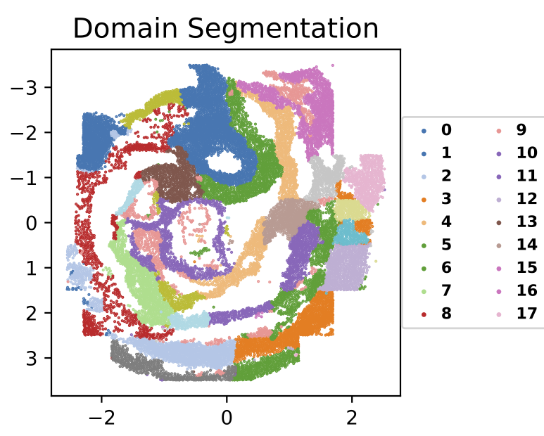
SpaceFlow will use this learned embedding to identify the spatial domains based on Leiden algorithm.

sf.segmentation(domain_label_save_filepath="./domains.tsv", n_neighbors=50, resolution=1.0)

Parameters:

• domain_label_save_filepath: the file path for saving the identified domain labels. (default: "./domains.tsv")
• n_neighbors: the number of the nearest neighbors for each cell for constructing the graph for Leiden using the embedding as input. (default: 50)
• resolution: the resolution of the Leiden clustering, the larger the coarser of the domains. (default: 1.0)

7. Visualization of the annotation and the identified spatial domains

We next plot the spatial domains using the identified domain labels and spatial coordinates of cells.

sf.plot_segmentation(segmentation_figure_save_filepath="./domain_segmentation.pdf", colormap="tab20", scatter_sz=1., rsz=4., csz=4., wspace=.4, hspace=.5, left=0.125, right=0.9, bottom=0.1, top=0.9)

The expected output is:

Parameters:

• segmentation_figure_save_filepath: optional, type: str, the file path for saving the figure of the spatial domain visualization. (default: "./domain_segmentation.pdf")
• colormap: optional, type: str, the colormap of the different domains, full colormap options see matplotlib
• scatter_sz: optional, type: float, the marker size in points. (default: 1.0)
• rsz: optional, type: float, row size of the figure in inches, (default: 4.0)
• csz: optional, type: float, column size of the figure in inches, (default: 4.0)
• wspace: optional, type: float, the amount of width reserved for space between subplots, expressed as a fraction of the average axis width (default: 0.4)
• hspace: optional, type: float,the amount of height reserved for space between subplots, expressed as a fraction of the average axis height (default: 0.4)
• left: optional, type: float, the leftmost position of the subplots of the figure in fraction (default: 0.125)
• right: optional, type: float, the rightmost position of the subplots of the figure in fraction (default: 0.9)
• bottom: optional, type: float, the bottom position of the subplots of the figure in fraction (default: 0.1)
• top: optional, type: float, the top position of the subplots of the figure in fraction (default: 0.9)

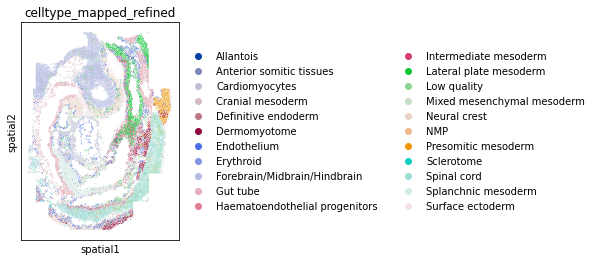
We can also visualize the expert annotation for comparison by:

import scanpy as sc
sc.pl.spatial(adata, color="celltype_mapped_refined", spot_size=0.03)

The expected output is:

8. Idenfify the spatiotemporal patterns of the ST data through pseudo-Spatiotemporal Map (pSM)

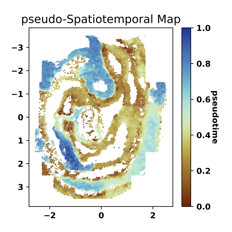
Next, we apply the diffusion pseudotime (dpt) algorithm to the learned spatially-consistent embedding to generate a pseudo-Spatiotemporal Map (pSM). This pSM represents a spatially-coherent pseudotime ordering of cells that encodes biological relationships between cells, such as developmental trajectories and cancer progression

sf.pseudo_Spatiotemporal_Map(pSM_values_save_filepath="./pSM_values.tsv", n_neighbors=20, resolution=1.0)

Parameters:

• pSM_values_save_filepath : the file path for saving the inferred pSM values.
• n_neighbors: the number of the nearest neighbors for each cell for constructing the graph for Leiden using the embedding as input. (default: 20)
• resolution: the resolution of the Leiden clustering, the larger the coarser of the domains. (default: 1.0)

9. Visualization of the identified pseudo-Spatiotemporal Map (pSM)

We next visualize the identified pseudo-Spatiotemporal Map (pSM).

sf.plot_pSM(pSM_figure_save_filepath="./pseudo-Spatiotemporal-Map.pdf", colormap="roma", scatter_sz=1., rsz=4., csz=4., wspace=.4, hspace=.5, left=0.125, right=0.9, bottom=0.1, top=0.9)

The expected output is:

Parameters:

• pSM_figure_save_filepath: optional, type: str, the file path for saving the figure of the pSM visualization. (default: "./pseudo-Spatiotemporal-Map.pdf")
• colormap: optional, type: str, the colormap of the pSM (default: 'roma'), full colormap options see Scientific Colormaps
• scatter_sz:optional, type: float, the marker size in points. (default: 1.0)
• rsz: optional, type: float, row size of the figure in inches, (default: 4.0)
• csz: optional, type: float, column size of the figure in inches, (default: 4.0)
• wspace: optional, type: float, the amount of width reserved for space between subplots, expressed as a fraction of the average axis width (default: 0.4)
• hspace: optional, type: float,the amount of height reserved for space between subplots, expressed as a fraction of the average axis height (default: 0.4)
• left: optional, type: float, the leftmost position of the subplots of the figure in fraction (default: 0.125)
• right: optional, type: float, the rightmost position of the subplots of the figure in fraction (default: 0.9)
• bottom: optional, type: float, the bottom position of the subplots of the figure in fraction (default: 0.1)
• top: optional, type: float, the top position of the subplots of the figure in fraction (default: 0.9)

Please cite

Ren, Honglei, et al. "Identifying multicellular spatiotemporal organization of cells with SpaceFlow." Nature Communications 13.1 (2022): 1-14. https://www.nature.com/articles/s41467-022-31739-w

Contact

If you have any questions or found any issues, please contact: [e-mail].