The goal of roadworksUK is to enable you to access, process and visualis data on UK roadworks, particularly Electronic Transfer of Notifications (EToN) records.
Install the package hosted on GitHub with:
# install.packages("devtools")
devtools::install_github("ITSLeeds/roadworksUK")
Load the package with:
library(roadworksUK)There are a number of functions for processing EToN records, as shown by:
x <- library(help = roadworksUK)
x$info[[2]]
#>  [1] "highway_authorities     Highway authorities"
#>  [2] "htdd_ashford            EtON roadworks data (raw HTDD logs from Elgin)"
#>  [3] "msoa_ashford            msoa boundary data for ashford"
#>  [4] "road_stats              Road statistics for HAs"
#>  [5] "rw_clean                clean roadworks data"
#>  [6] "rw_clean_points         Clean Spatial Part of the HDDT Data"
#>  [7] "rw_import_elgin_batch   Bulk Import Elgin road works data"
#>  [8] "rw_import_elgin_ed      Import Elgin ED road works data"
#>  [9] "rw_import_elgin_htdd    Import Elgin HDDT road works data"
#> [10] "rw_import_elgin_restrictions"
#> [11] "                        Import Elgin Restrictions road works data"
#> [12] "rw_import_elgin_ttvdd   Import Elgin TTVDD road works data"
#> [13] "rw_import_scot          Import Scottish road works data"
#> [14] "rw_points_to_region     Match Points to Regions"
#> [15] "rw_spatial              Convert an data frame containing roadworks data"
#> [16] "                        into a spatial data object"
#> [17] "rw_spec_scottish        Scottish road works spec"
The datasets provided by the package include kent10, a minimal dataset
containing data from Kent, htdd_ashford, ~981 records from Ashford,
Kent. The characteristics of these datasets is demonstrated below:
data("htdd_ashford")
dim(htdd_ashford) # a larger dataset
#> [1] 981  90
htdd_ashford[1:3, 1:5]
#>           id entity_id item_id                works_ref project_ref
#> 446 38017881 105824835 4187672          EB006-M16861611
#> 447 38017882 105824859 4187693              GE605218822
#> 525 38017960 105860399 4211964 GE4000ENT000000058915491
file_path = system.file("extdata", "kent10.csv.gz", package = "roadworksUK")
file.exists(file_path)
#> [1] TRUE
htdd_example = rw_import_elgin_htdd(file_path = file_path)
ncol(htdd_example)
#> [1] 91
nrow(htdd_example) # a small dataset with 10 rows
#> [1] 10This section explores roadworks htdd_ashford, a dataset that is
provided by the package: it’s made available when you load
roadworksUK. It relies on the tidyverse:
library(tidyverse)A good way to ‘get the measure’ of potentially large spatio-temporal
datasets is to find their size (in MB/GB/TB and number of rows/columns)
and their temporal extent (we’ll plot its spatial extent soon). We can
find all of these things for the htdd_ashford dataset as follows:
pryr::object_size(htdd_ashford) # less than 2 MB - good test dataset
#> 1.65 MB
nrow(htdd_ashford)
#> [1] 981
ncol(htdd_ashford)
#> [1] 90
range(htdd_ashford$e__date_created)
#> [1] "2018-01-31 13:35:31 UTC" "2018-07-26 09:33:05 UTC"
A summary table of the contents of this dataset can be generated as follows:
htdd_ashford %>%
  select(id, responsible_org_name, responsible_org_sector, description) %>%
  slice(1:10) %>%
knitr::kable()| id | responsible_org_name | responsible_org_sector | description |
|---|---|---|---|
| 38017881 | South East Water | Water | CUSTOMER METER INSTALLATION |
| 38017882 | KENT COUNTY COUNCIL | Highway Authority | COLUMN REPLACEMENT |
| 38017960 | KENT COUNTY COUNCIL | Highway Authority | FAO ANDY GODDEN EVEGATE MILL LANE PRE PATCHING FOR SURFACE DRESSING IN ACORDANCE WITH THE TRAFFIC SIGNS MANUAL CHAPTER 8 FROM SMALL STREAM TO CALLEYWELL LANE - FAO ANDY GODDEN EVEGATE MILL LANE PRE PATCHING FOR SURFACE DRESSING IN ACCORDANCE WITH THE |
| 38017988 | Highways England | Highway Authority | |
| 38018147 | KENT COUNTY COUNCIL | Highway Authority | CW Patch |
| 38018184 | KENT COUNTY COUNCIL | Highway Authority | CW Potholes |
| 38018288 | KENT COUNTY COUNCIL | Highway Authority | Crew to take up to tip one number gully grate and demolish the existing brick-built gully. |
| 38018532 | KENT COUNTY COUNCIL | Highway Authority | Crew req’d to repair 2no. C/way patches located at the give way markings 1) 1.4m x 0.9m x 40mm. 2) 1.6m x 1m x 40mm. |
| 38018734 | South East Water | Water | REPAIR COMM PIPE - CONTRACTOR DAMAGE |
| 38019363 | South East Water | Water | COMM PIPE REPAIR |
The following commands can find-out who reports road works in Ashford, using the dplyr package (part of the tidyverse):
htdd_ashford %>%
  group_by(publisher_name) %>%
  summarise(n = n()) %>%
  arrange(desc(n))
#> # A tibble: 2 x 2
#>   publisher_name          n
#>   <chr>               <int>
#> 1 Kent County Council   975
#> 2 Highways England        6
It’s mostly Kenty County Council. There are a handful of reports by HE
in the region also. Find out who does the work with the following
commands (this finds the top 5 organisations, change then n parameter
to see more organisations):
htdd_ashford %>%
  group_by(responsible_org_name) %>%
  summarise(n = n()) %>%
  arrange(desc(n)) %>%
  top_n(n = 5, wt = n)
#> # A tibble: 5 x 2
#>   responsible_org_name                n
#>   <chr>                           <int>
#> 1 KENT COUNTY COUNCIL               528
#> 2 South East Water                  273
#> 3 BT                                 47
#> 4 UK POWER NETWORKS SOUTH EASTERN    38
#> 5 SOUTHERN GAS NETWORKS              24
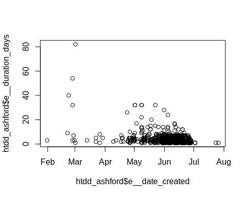
Let’s take a look at the temporal distribution of roadworks in the example dataset:
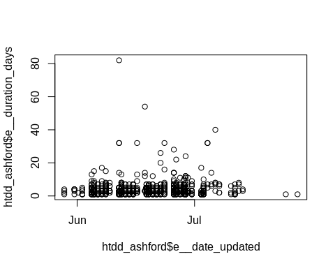
plot(htdd_ashford$e__date_created, htdd_ashford$e__duration_days)This distribution is characteristic of roadworks data: it’s not usually logged when it begins but after it ends. A log of actual reporting dates is illustrated in the next plot:
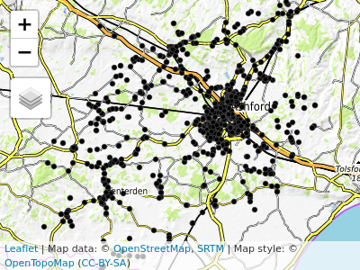
plot(htdd_ashford$e__date_updated, htdd_ashford$e__duration_days)This shows the log comes from a single month (June) in 2018. We can do more sophisticated plots building on these examples and using packages such as ggplot2. For now, we will move on to plot the spatial extent of the object:
library(tmap)
tmap_mode("view")
#> tmap mode set to interactive viewing
tm_basemap(server = leaflet::providers$OpenTopoMap) +
  qtm(htdd_ashford$i__location_point)
#> Linking to GEOS 3.6.2, GDAL 2.2.3, proj.4 4.9.3library(tidyverse)
htdd_small = htdd_ashford %>%
select(description)

