Histogrammar is a declarative grammar for booking histograms with automatic filling and merging. It simplifies the process of reducing a huge, distributed dataset to a form that can be plotted, especially in a functional workflow like Apache Spark. It is a standardized set of routines available in many programming languages that interoperate by serializing to and from JSON. It also generalizes the concept of histogramming to an algebra of composable primitives, allowing them to be combined in novel ways.
That was the concise overview. Here's a simple example.
import org.dianahep.histogrammar._
import org.dianahep.histogrammar.histogram._

val px_histogram = Histogram(100, -5, 5, {mu: Muon => mu.px})
val pt_histogram = Histogram(80, 0, 8, {mu: Muon => Math.sqrt(mu.px*mu.px + mu.py*mu.py)})
val cut_histogram = Histogram(100, -5, 5, {mu: Muon => mu.px}, {mu: Muon => mu.py < 0.0})

val all_histograms = Label("px" -> px_histogram, "pt" -> pt_histogram, "cut" -> cut_histogram)

val final_histogram = rdd.aggregate(all_histograms)(new Increment, new Combine)

println(final_histogram("pt").ascii)
The rdd.aggregate function submits the histograms to Spark, which fills independent partial histograms in each of its worker nodes, combines partial results, and returns the final result for plotting. However, it required very little input from the user. In this example, rdd is a dataset of Muon objects, which the histograms view in different ways.
Most of the code in this snippet is concerned with booking the histograms (setting the range and number of bins) and describing how to fill them with data. The fill rule is given in each histogram's constructor, so that the data analyst doesn't have to maintain the booking in one part of the code, filling in another, and (for distributed jobs) combining in yet another part of the code. In a data analysis with hundreds of histograms, rather than three, this consolidation helps considerably.
The all_histograms object in the example above is a mapping from names to histograms. It, too, has a booking-incrementing-combining lifecycle, where its fill rule is to pass all of the data to all of its constituents. It is a sort of "meta-histogram," an aggregator of aggregators.
We could orgnize the histograms into directories by nesting them, because Label classes are composable:
val directories = Label("momentum" -> Label("px" -> ..., "pt" -> ...),
"position" -> Label("x" -> ..., "y" -> ...))But what if we wanted to make a histogram of histograms? That is, something like the following:
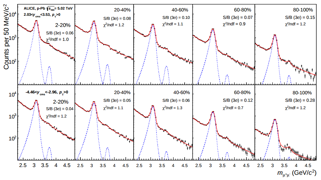
(source)
The top row of plots show data in one region of y (rapidity), the bottom show another; each column shows data in a different "bin" of centrality, and the plots themselves are histograms of m (dimuon mass).
Just as we could make directories by nesting the Label class, we should be able to make multivariate views of a dataset by nesting histograms. But to do that effectively, we have to decompose histograms into their fundamental components.
A histogram is a summary of a dataset, produced by aggregation. There are other ways to summarize a dataset by aggregation: simply counting the number of entries, computing the sum of some quantity, computing a mean or standard deviation, etc. Each of these summarizes the data in a different way, conveying more or less information.
A histogram is a continuous variable that has been discretized (binned) and the number of entries in each bin are simply counted. Thus, we could write a histogram aggregator like this:
val histogram = Bin(numberOfBins, low, high, fillRule, value = Count())The Bin is a container of sub-aggregators, much like Label, but its behavior is different. Now consider the following.
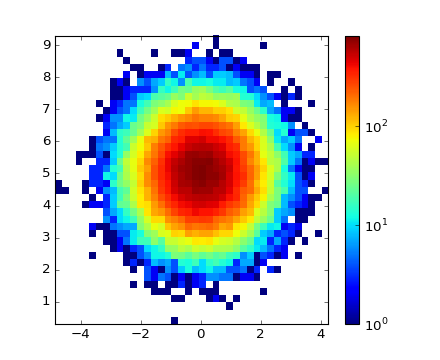
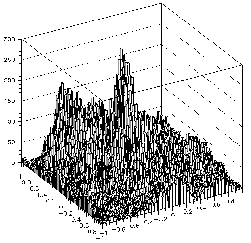
val h2d = Bin(numBinsX, lowX, highX, fillX, value = Bin(numBinsY, lowY, highY, fillY, value = Count())This aggregator divides the space by binning in one continuous variable, X, and then further subdivides it by binning in Y Then it counts. The result is a two-dimensional histogram, like both of the following:
(left source: matplotlib) (right source: PAW)
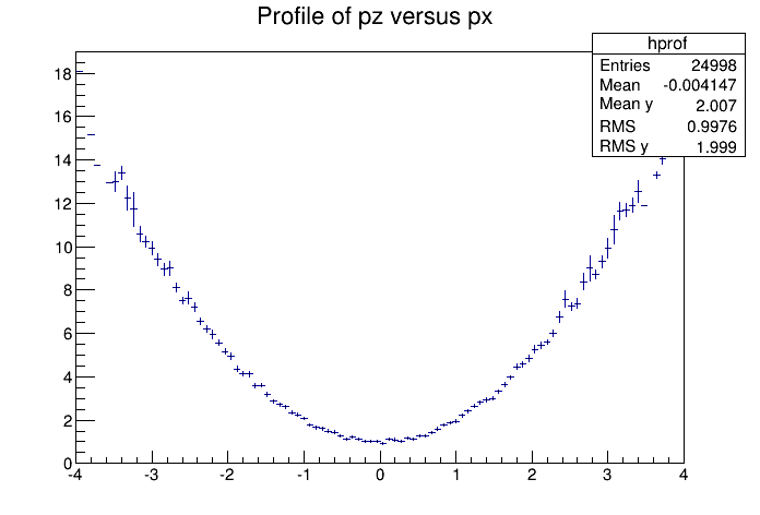
A so-called "profile plot" is a histogram in which each bin accumulates a mean and standard deviation, rather than a count. The Histogrammar primitive for mean and standard deviation is Deviate.
val profile = Bin(numBinsX, lowX, highX, fillRuleX, value = Deviate(fillRuleY))The appropriate set of primitives can make short work of many common plot types. Most of these are often assembled by hand.
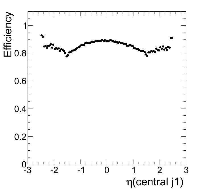
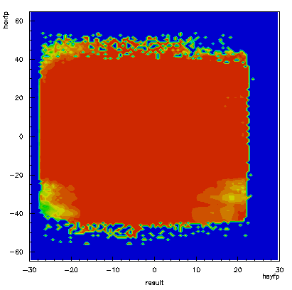
val efficiency = Fraction({mu: Muon => mu.passesTrigger}, Histogram(120, -2.4, 2.4, {mu: Muon => mu.eta})val efficiency2d = Fraction({mu: Muon => mu.passesTrigger},
Bin(100, -30, 30, {mu: Muon => mu.x}, value =
Bin(100, -60, 60, {mu: Muon => mu.y}, value = Count())))Histogram bins turn a numerical feature into categories. But sometimes the data are already categorical.
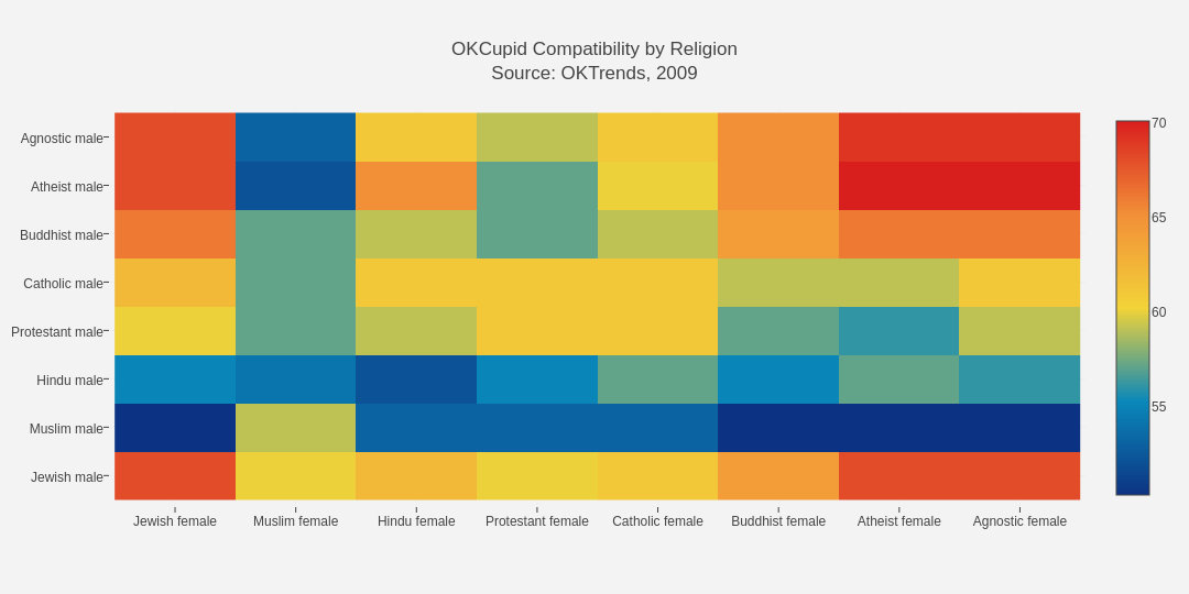
val categorical_heatmap = Categorize({d: D => d.femaleReligion}, value =
Categorize({d: D => d.maleReligion}, value = Count())And that allows us to freely mix categorical and numerical aggregation.
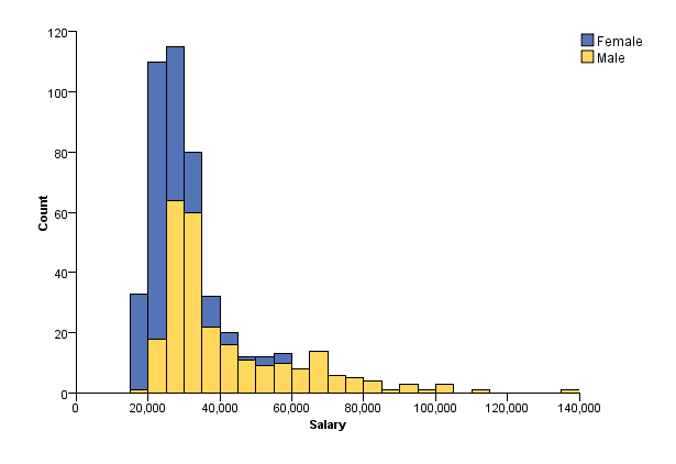
val mixed = CategoricalStack(Histogram(140, 0, 140000, {d: D => d.salary}), {d: D => d.gender})It also lets us swap one binning strategy with another without affecting anything else in the hierarchy.
- Bin: user specifies number of bins, low edge, and high edge; bins are regularly spaced.
- SparselyBin: user specifies bin width; bins are filled when non-zero using a hash-map (still regularly spaced).
- CentrallyBin: user specifies bin centers, which may be irregularly spaced. Membership is determined by closest center, which makes histogramming a close analogue of clustering in one dimension.
- AdaptivelyBin: user specifies nothing; optimal bin placement is determined by a clustering algorithm.
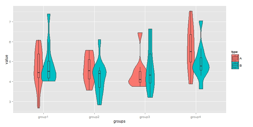
The last is particularly useful for exploratory analysis: you want to make a plot to understand the distribution of your data, but specifying bins relies on prior knowledge of that distribution. It is also an essential ingredient in estimating medians and quartiles for box-and-whiskers plots, or mini-histograms for violin plots.
val violin_box = Branch(Categorize({d: D => d.group}, value = AdaptivelyBin({d: D => d.value}),
Categorize({d: D => d.group}, value = Quantile({d: D => d.value}))))In the discussion above, I included plots from many different plotting packages. Histogrammar is not a plotting package: it aggregates data and passes the result to your favorite plotter. Usually, the aggregation step is more computationally expensive than plotting, so it's frustrating to have to repeat a time-consuming aggregation just to change a cosmetic aspect of a plot. Aggregation and graphics must be kept separate.
Aggregation primitives are also easier to implement than graphics, so Histogrammar's core of primitives will be implemented in many different programming languages with a canonical JSON representation. A dataset aggregated in Scala can be plotted in Python. Most language-specific implementations recognize common patterns, such as bin-count being a one-dimensional histogram, to generate the appropriate plot.
Zeroth kind: primitives that ignore data and depend only on weights.
- Count: Count data, ignoring their content. (Actually a sum of weights.)
First kind: primitives that aggregate a given scalar quantity, without sub-aggregators.
- Sum: Accumulate the sum of a given quantity.
- Average: Accumulate the weighted mean of a given quantity.
- Deviate: Accumulate a weighted variance, mean, and total weight of a given quantity (using an algorithm that is stable for large numbers).
- AbsoluteErr: Accumulate the weighted Mean Absolute Error (MAE) of a quantity whose nominal value is zero.
- Minimize: Find the minimum value of a given quantity. If no data are observed, the result is NaN.
- Maximize: Find the maximum value of a given quantity. If no data are observed, the result is NaN.
- Quantile: Estimate a quantile, such as 0.5 for median, (0.25, 0.75) for quartiles, or (0.2, 0.4, 0.6, 0.8) for quintiles.
Second kind: primitives that group by a given scalar quantity, passing data to a sub-aggregator.
- Bin: Split a given quantity into equally spaced bins between specified limits and fill only one bin per datum.
- SparselyBin: Split a quantity into equally spaced bins, filling only one bin per datum and creating new bins as necessary.
- CentrallyBin: Split a quantity into bins defined by a set of bin centers, filling only one datum per bin with no overflows or underflows.
- AdaptivelyBin: Split a quanity into bins dynamically with a clustering algorithm, filling only one datum per bin with no overflows or underflows.
- Categorize: Split a given quantity by its categorical (string-based) value and fill only one category per datum.
- Fraction: Accumulate two containers, one with all data (denominator), and one with data that pass a given selection (numerator).
- Stack: Accumulate a suite containers, filling all that are above a given cut on a given expression.
- Partition: Accumulate a suite containers, filling the one that is between a pair of given cuts on a given expression.
Third kind: primitives that act as containers, passing data to all sub-aggregators.
- Cut: Accumulate an aggregator for data that satisfy a cut (or more generally, a weighting).
- Limit: Accumulate an aggregator until its number of entries reaches a predefined limit.
- Label: Accumulate any number of containers of the SAME type and label them with strings. Every one is filled with every input datum.
- UntypedLabel: Accumulate containers of any type except Count and label them with strings. Every one is filled with every input datum.
- Index: Accumulate any number of containers of the SAME type anonymously in a list. Every one is filled with every input datum.
- Branch: Accumulate containers of DIFFERENT types, indexed by i0 through i9. Every one is filled with every input datum.
Fourth kind: primitives that collect sets of raw data.
- Bag: Accumulate raw numbers, vectors of numbers, or strings, merging identical values.
- Sample: Accumulate raw numbers, vectors of numbers, or strings that are an unbiased sample of the observed distribution.
Last released version was 0.5. The following refers to the git master branch.
| Primitive | Scala | Python (undocumented) | C++ | CUDA (Python) | CUDA/OpenCL | R | Javascript | SQL |
|---|---|---|---|---|---|---|---|---|
| Count | done | done | done | |||||
| Sum | done | done | done | |||||
| Average | done | done | ||||||
| Deviate | done | done | ||||||
| AbsoluteErr | done | done | ||||||
| Minimize | done | done | ||||||
| Maximize | done | done | ||||||
| Quantile | done | done | ||||||
| Bin | done | done | done | |||||
| SparselyBin | done | done | ||||||
| CentrallyBin | done | done | ||||||
| AdaptivelyBin | done | done | ||||||
| Categorize | done | done | ||||||
| Fraction | done | done | ||||||
| Stack | done | done | ||||||
| Partition | done | done | ||||||
| Cut | done | |||||||
| Limit | done | done | ||||||
| Label | done | done | ||||||
| UntypedLabel | done | done | ||||||
| Index | done | done | ||||||
| Branch | done | done | ||||||
| Bag | done | done | ||||||
| Sample | done |
Needs to be synchronized: Scala has
- selection functions removed from all primitives except Cut and Fraction: express cuts by composing;
- the Histogram convenience function is now Cut(Bin(Count())), which changes the Histogram methods;
- user functions have (implicit) methods to add names and cache functionality;
- function name is propagated through JSON if it exists;
and Python needs to get these features. Same for C++. Cut will need to be the third primitive implemented.
Think about a rollback feature: if an exception occurs during filling, the state should rollback to what it had been just before the fill attempt. Is this too hard for all languages (C++)?
