\begin{titlepage}
\begin{center}
\line(1,0){300}
[5mm]
\huge{\bfseries Differential Equations Coursework} \
\huge{Aeroplane Landing Modelling} \
[5mm]
\huge{Gleb Dianov} \
\end{center}
\end{titlepage}
\newpage
\tableofcontents
\newpage
Simplifying situation and setting up the model
Given data
I’ve been given data about a landing aeroplane after touchdown. The mass of the aeroplane is
| t | v | t | v |
|---|---|---|---|
| 0 | 96 | 14 | 34 |
| 1 | 89 | 15 | 31 |
| 2 | 82 | 16 | 27 |
| 3 | 77 | 17 | 24 |
| 4 | 72 | 18 | 21 |
| 5 | 68 | 19 | 18 |
| 6 | 64 | 20 | 16 |
| 7 | 61 | 21 | 13 |
| 8 | 58 | 22 | 10 |
| 9 | 55 | 23 | 8 |
| 10 | 50 | 24 | 5 |
| 11 | 46 | 25 | 3 |
| 12 | 41 | 26 | 0 |
| 13 | 38 |
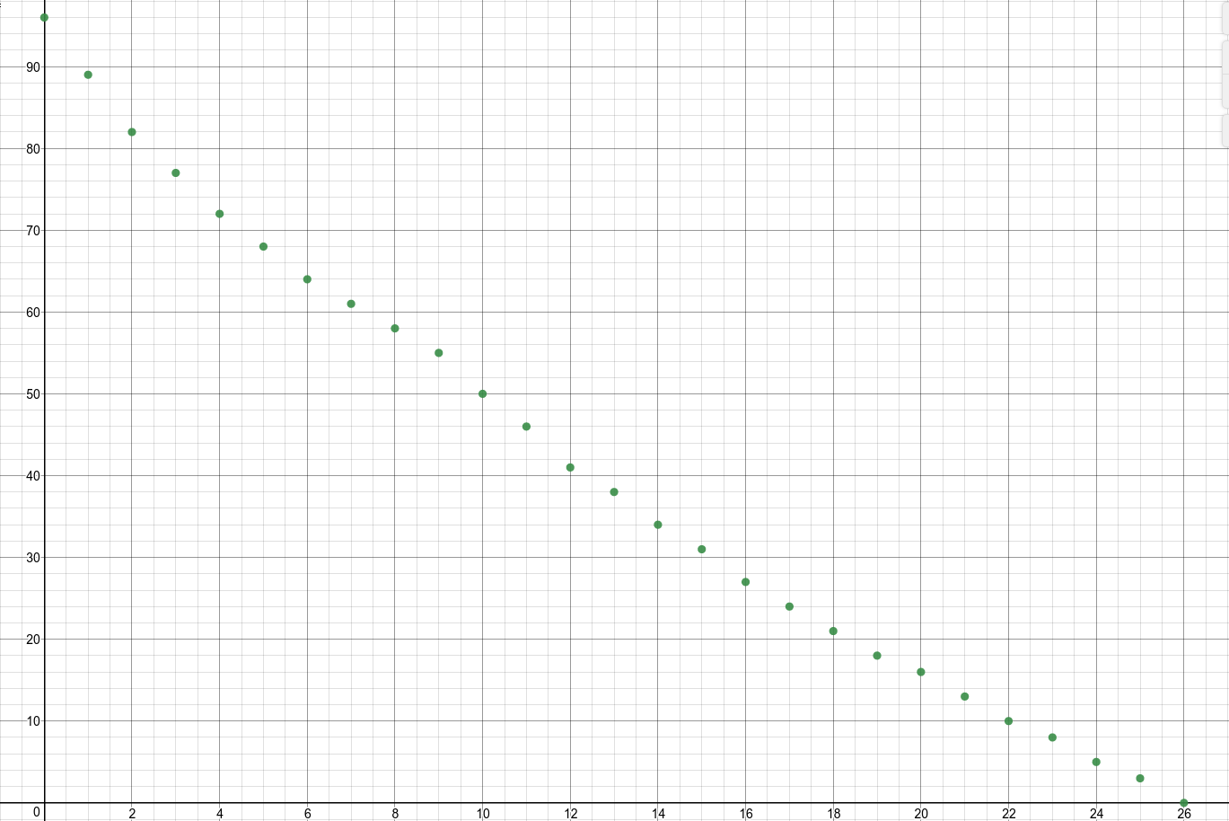
The image below shows a chart of the original data.
Modeling assumptions
- The aeroplane can be modeled as a point particle. This assumption allows us to negate any complex resistances that would occur. Modeling this way is appropriate because we are not given velocity (only speed) of the aeroplane at different points in time, so we are not interested in any rotations of the plane.
- The runway can be modeled as a plane. Without this assumption we would need to consider the possibility that the runway has a complex shape, for example it can have hills and/or pits.
- The runway is horizontal. Without this assumption we would need to include components of the weight and the reaction force in the model which would increase the complexity of the model and affect the calculations.
- The aeroplane is moving in the horizontal plane. This assumption allows us to negate any vertical forces.
- The constant force from the wheel brakes (after the brakes are applied) and the air resistance are the only forces acting on the aeroplane in the horizontal plane. This assumption allows us to say that any other resistance is negligible and there are no other forces, alternatively we can say that the air resistance model is a model of the total resistance force.
-
The given values for speed are rounded to the nearest integer. This assumption allows the model of speed to have an error
$±0.5$ . It’s very unlikely that the values of speed are exactly integers, so it’s a reasonable assumption. -
Brakes are applied at $t = 9$. The table below shows differences between consecutive speed values,
$Δ v$ , and differences between consecutive differences,$Δ (Δ v)$ .$Δ (Δ v)$ is the lowest when$t = 10$ . This means that the highest decrease of acceleration occurred between$t = 9$ and$t = 10$ , hence we will assume that the brakes were applied during that time. We will model this as if the brakes were applied at$t = 9$ .
| t | v | Δ v | Δ (Δ v) | t | v | Δ v | Δ (Δ v) |
|---|---|---|---|---|---|---|---|
| 0 | 96 | 14 | 34 | -4 | -1 | ||
| 1 | 89 | -7 | 15 | 31 | -3 | 1 | |
| 2 | 82 | -7 | 0 | 16 | 27 | -4 | -1 |
| 3 | 77 | -5 | 2 | 17 | 24 | -3 | 1 |
| 4 | 72 | -5 | 0 | 18 | 21 | -3 | 0 |
| 5 | 68 | -4 | 1 | 19 | 18 | -3 | 0 |
| 6 | 64 | -4 | 0 | 20 | 16 | -2 | 1 |
| 7 | 61 | -3 | 1 | 21 | 13 | -3 | -1 |
| 8 | 58 | -3 | 0 | 22 | 10 | -3 | 0 |
| 9 | 55 | -3 | 0 | 23 | 8 | -2 | 1 |
| 10 | 50 | -5 | -2 | 24 | 5 | -3 | -1 |
| 11 | 46 | -4 | 1 | 25 | 3 | -2 | 1 |
| 12 | 41 | -5 | -1 | 26 | 0 | -3 | -1 |
| 13 | 38 | -3 | 2 |
- Braking force starts working instantly. This assumption makes acceleration not continuous and simplifies the calculations.
- There is no wind. This allows us to assume that if the plane is not moving then there is no air resistance.
\newpage
Derivation of the initial model
The diagram shows the x-axis, direction of velocity,
Model 1
Defining f(v)
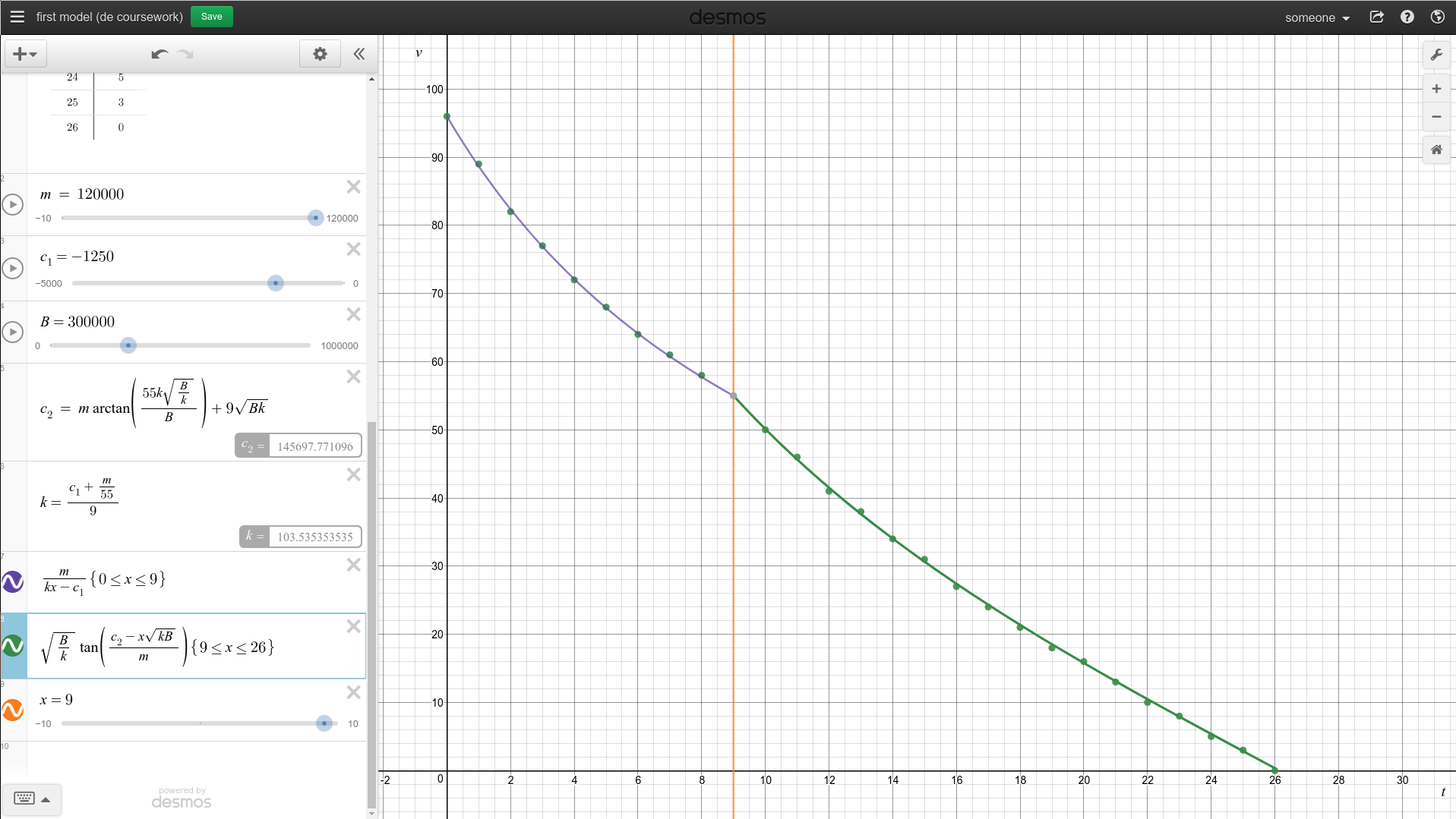
As you can see in the table with the differences, speed for
To make
General solution
0 \leq t \leq 9
9 \leq t \leq 26
Particular solution
The general solution has 4 unknown constants: the constant braking force,
$$ \begin{cases} \frac{m}{9k - c_1} = 55 \ \sqrt{\frac{B}{k}} tan \frac{c_2 - 9\sqrt{kB}}{m} = 55 \end{cases} $$
$$ ⇒ 9k - c_1 = \frac{m}{55} $$
$$ ⇒ k = \frac{c_1 + \frac{m}{55}}{9} $$
$$ S \mbox{ is the set of given data.} $$
$$ (t_1, v_1), (t_2, v_2) ∈ S; t_1, t_2 \leq 9, t_1 ≠ t_2 $$
$$ \begin{cases} v_1 = \frac{m}{t_1k - c_1} \ v_2 = \frac{m}{t_2k - c_1} \end{cases} $$
$$ ⇒ \begin{cases} v_1v_2t_2t_1k - v_1v_2t_2c_1 = mv_2t_2 \ v_1v_2t_1t_2k - v_1v_2t_1c_1 = mv_1t_1 \end{cases} $$
$$ ⇒ c_1v_1v_2(t_2 - t_1) = m(v_1t_1 - v_2t_2) $$
$$ ⇒ c_1 = \frac{m(v_1t_1 - v_2t_2)}{v_1v_2(t_2 - t_1)} $$
$$ \sqrt{\frac{B}{k}} tan \frac{c_2 - 9\sqrt{kB}}{m} = 55 $$
$$ ⇒ c_2(B) = marctan(\frac{55k\sqrt{\frac{B}{k}}}{B}) + 9\sqrt{Bk} $$
$$ (t_3, v_3) ∈ S; t_3 > 9 $$
$$ ⇒ v_3 = \sqrt{\frac{B}{k}} tan \frac{c_2(B) - \sqrt{kB}t_3}{m} $$
$$ ⇒ arctan(v_3\sqrt{\frac{k}{B}}) = \frac{c_2(B) - \sqrt{kB}t_3}{m} $$
$$ \mbox{Let } λ(B) = \frac{c_2(B) - \sqrt{kB}t_3}{m} - arctan(v_3\sqrt{\frac{k}{B}}) $$
$$ \mbox{Newton-Raphson’s rule: } Bn+1 = B_n + \frac{λ’(B_n)}{λ(B_n)} $$
\begin{equation}
\begin{cases}
c_1 = \frac{m(v_1t_1 - v_2t_2)}{v_1v_2(t_2 - t_1)}
k = \frac{c_1 + \frac{m}{55}}{9} \
c_2(B) = marctan(\frac{55k\sqrt{\frac{B}{k}}}{B}) + 9\sqrt{Bk} \
λ(B) = \frac{c_2(B) - \sqrt{kB}t_3}{m} - arctan(v_3\sqrt{\frac{k}{B}}) \
Bn+1 = B_n - \frac{λ(B_n)}{λ’(B_n)}
B_0 = 300000
\end{cases}
\end{equation}
To find
Now I can use programming to find the parameters. To do this I wrote 5 modules in Haskell. The first module is a module for automatic differentiation using dual numbers and Newton-Raphson method.
The second module contains the given data.
\newpage
Then I defined a general interface for models.
The fourth module is for the first model and finding parameters.
And finally the main module, which runs this code to find the parameters.
import           Data.List      (sort, sortOn)
import           Data.Proxy

import           GivenData
import qualified Solution.First as Sol
import           Solution.Model as Model

adjustLength :: (a -> String) -> (a -> String -> b) -> [a] -> [b]
adjustLength g s l =
  (\x -> let str = g x in s x $ str ++ replicate (longest - length str) ' ') <$> l
  where longest = maximum $ length . g <$> l

showPredictions :: (ModelParams f, Show (f Double)) => f Double -> String
showPredictions params =
  foldMap (\(x, y, z, w) -> "| " ++ x ++ " | " ++ y ++ " | " ++ z ++ " | " ++ w ++ " |\n")
     $  adjustLength (\(_, _, _, w) -> w) (\(x, y, z, _) w -> (x, y, z, w))
     $  adjustLength (\(_, _, z, _) -> z) (\(x, y, _, w) z -> (x, y, z, w))
     $  adjustLength (\(_, y, _, _) -> y) (\(x, _, z, w) y -> (x, y, z, w))
     $  adjustLength (\(x, _, _, _) -> x) (\(_, y, z, w) x -> (x, y, z, w))
     $  (("Time", "Predicted Speed", "Rounded predicted speed", "Observed Speed"):)
     $  (\(Point t v) -> let v' = predict params t in (show t, show v', rounded v', rounded v))
    <$> points
  where rounded = show . round

maxErr :: (a -> Double -> Double) -> a -> Double
maxErr predict params =
  maximum $ abs . (\(Point t v) -> predict params t - v) <$> points
  where n = fromIntegral (length points)

avrErr :: (a -> Double -> Double) -> a -> Double
avrErr predict params =
  (/ n) $ sum $ abs . (\(Point t v) -> predict params t - v) <$> points
  where n = fromIntegral (length points)

rms :: (a -> Double -> Double) -> a -> Double
rms predict params =
  (/ n) $ sqrt $ sum $ (^2) . (\(Point t v) -> predict params t - v) <$> points
  where n = fromIntegral (length points)

showErrors :: (ModelParams f, Show (f Double)) => f Double -> String
showErrors params =
  foldMap (\(x, y, z) -> "| " ++ x ++ " | " ++ y ++ " | " ++ z ++ " |\n")
  $  adjustLength (\(_, _, z) -> z) (\(x, y, _) z -> (x, y, z))
  $  adjustLength (\(_, y, _) -> y) (\(x, _, z) y -> (x, y, z))
  $  adjustLength (\(x, _, _) -> x) (\(_, y, z) x -> (x, y, z))
  [ ("Maximum Error", "Average Error", "Root mean square")
  , (show $ maxErr predict params, show $ avrErr predict params, show $ rms predict params)
  ]

showResults :: (ModelParams f, Show (f Double)) => f Double -> String
showResults params = show params ++ "\n"
                  ++ showErrors params ++ "\n"
                  ++ showPredictions params

results :: [Sol.Parameters Double]
results =  sortOn (rms predict) $ findParams
      <$> combinations (Proxy :: Proxy Sol.Parameters)

main :: IO ()
main = do putStrLn "The best result:"
          putStrLn $ showResults $ head results
          putStrLn "The worst result:"
          putStr   $ showResults $ last results
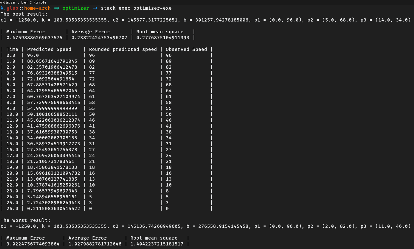
Here is the result. It shows the best and the worst parameters found using the derived formulas and for both of the configurations it shows sums of squares of errors, and predictions for each of the given point with rounded versions.
Graphs and Analysis
| Time | Predicted | Rounded | Observed |
| Speed | Predicted | Speed | |
| Speed | |||
|---|---|---|---|
| 0.0 | 96.0 | 96 | 96 |
| 1.0 | 88.65671641791045 | 89 | 89 |
| 2.0 | 82.35701906412478 | 82 | 82 |
| 3.0 | 76.89320388349515 | 77 | 77 |
| 4.0 | 72.1092564491654 | 72 | 72 |
| 5.0 | 67.88571428571429 | 68 | 68 |
| 6.0 | 64.12955465587045 | 64 | 64 |
| 7.0 | 60.767263427109974 | 61 | 61 |
| 8.0 | 57.739975698663415 | 58 | 58 |
| 9.0 | 54.99999999999999 | 55 | 55 |
| 10.0 | 50.10816658852111 | 50 | 50 |
| 11.0 | 45.622063036212374 | 46 | 46 |
| 12.0 | 41.475988862696376 | 41 | 41 |
| 13.0 | 37.61659930730753 | 38 | 38 |
| 14.0 | 34.00002062308155 | 34 | 34 |
| 15.0 | 30.589724513917773 | 31 | 31 |
| 16.0 | 27.35493651754378 | 27 | 27 |
| 17.0 | 24.269426053394415 | 24 | 24 |
| 18.0 | 21.3105731783461 | 21 | 21 |
| 19.0 | 18.45863841578133 | 18 | 18 |
| 20.0 | 15.696183121094782 | 16 | 16 |
| 21.0 | 13.00760227741885 | 13 | 13 |
| 22.0 | 10.378741615250261 | 10 | 10 |
| 23.0 | 7.796577949697343 | 8 | 8 |
| 24.0 | 5.248946558956161 | 5 | 5 |
| 25.0 | 2.7243028986249413 | 3 | 3 |
| 26.0 | 0.2115083630415522 | 0 | 0 |
| Maximum Error | Average Error | Root mean square |
|---|---|---|
| 0.47598886269637575 | 0.23822424753496707 | 0.2776875104911393 |
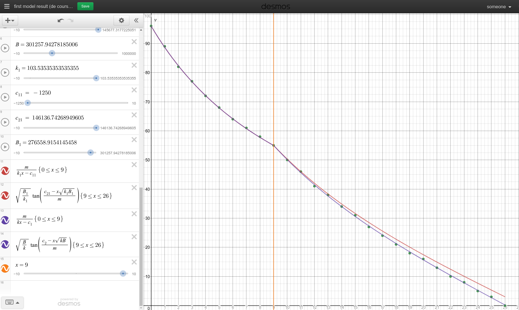
I’ll now look at the two configurations that I obtained and plot them. The red line shows the worst configuration, and the purple line shows the best configuration.
As you can see in first_model_code_result rounded predictions of the best configuration exactly match the given data.
Conclusion of Model 1
\begin{equation}
\begin{cases}
v(t) = \frac{m}{kt - c_1}, & 0 \leq t \leq 9
v(t) = \sqrt{\frac{B}{k}} tan(\frac{c_2 -\sqrt{kB}t}{m}), & 9 \leq t \leq 26 \
c_1 = -1250.0 \
k = 103.\dot{5}\dot{3} \
c_2 = 145677.3177225051 \
B = 301257.94278185006 \
\end{cases}
\end{equation}
The aeroplane fully stops in approximately
Model 2
Redefining f(v)
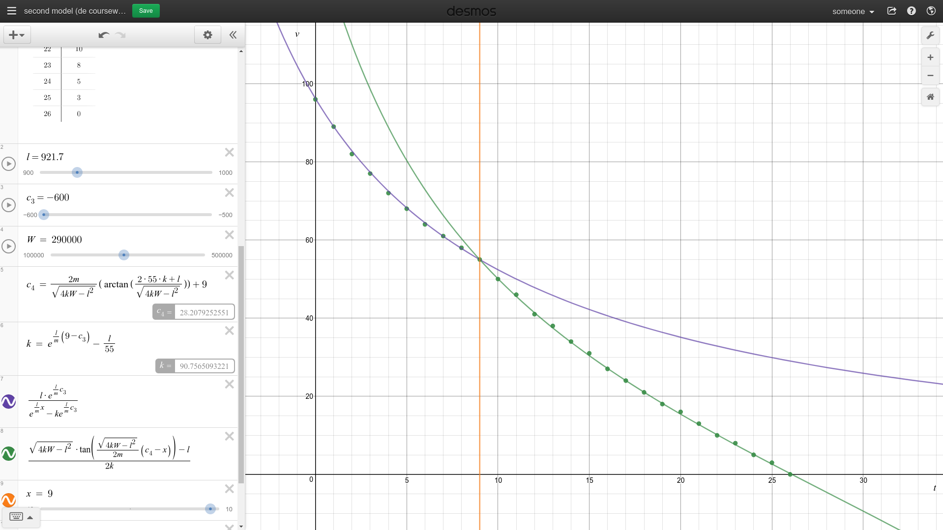
Although the first model fits the given data very well, I think this model can be improved. This time I will add a linear term to the air resistance function.
General solution
0 \leq t \leq 9
9 \leq t \leq 26
Particular solution
We want to minimize
I found
\begin{equation}
\begin{cases}
c_3 = \frac{m}{λ}ln(\frac{v_1v_2(e\frac{λ{m}t_1} - e\frac{λ{m}t_2})}{λ(v_2 - v_1)})
k = e\frac{λ{m}(9 - c_3)} - \frac{λ}{55} \
ζ(λ) = ∂λ∑(t,v) ∈ S, t \leq 9 (\frac{λ e\frac{λ{m} c_3}}{e\frac{λ{m} t} - ke\frac{λ{m}c_3}} - v)^2 \
λn+1 = λ_n - \frac{ζ(λ_n)}{ζ’(λ_n)} \
λ_0 = 921.7 \
c_4 = 9 + \frac{2marctan(\frac{110k + λ}{\sqrt{4kW - λ^2}})}{\sqrt{4kW-λ^2}} \
φ(W) = ∂_W ∑(t,v) ∈ S, t \geq 9 \left(\frac{\sqrt{4kW-λ^2}}{2m}(c_4 - t) - arctan(\frac{2kv + λ}{\sqrt{4kW - λ^2}})\right)^2 \
Wn+1 = W_n - \frac{φ(W)}{φ’(W)} \
W_0 = 290000
\end{cases}
\end{equation}
I wrote another module for the second model:
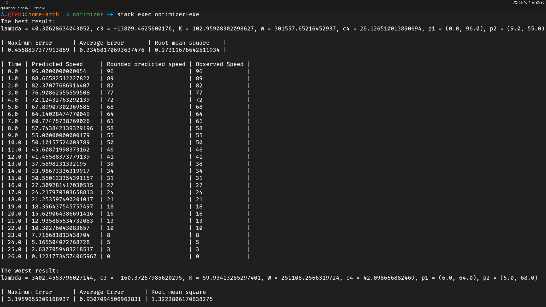
I also changed import Solution.First as Sol to import Solution.Second as Sol in the main module. This code gives us the following result:
Graphs and Analysis
| Time | Predicted | Rounded | Observed |
| Speed | Predicted | speed | |
| Speed | |||
|---|---|---|---|
| 0.0 | 96.0000000000054 | 96 | 96 |
| 1.0 | 88.66582512227822 | 89 | 89 |
| 2.0 | 82.37077686914407 | 82 | 82 |
| 3.0 | 76.90862555559508 | 77 | 77 |
| 4.0 | 72.12432763292139 | 72 | 72 |
| 5.0 | 67.89907302369585 | 68 | 68 |
| 6.0 | 64.14028474770049 | 64 | 64 |
| 7.0 | 60.77475738769026 | 61 | 61 |
| 8.0 | 57.743842139329196 | 58 | 58 |
| 9.0 | 55.00000000000179 | 55 | 55 |
| 10.0 | 50.10157524003789 | 50 | 50 |
| 11.0 | 45.60871998373162 | 46 | 46 |
| 12.0 | 41.45588373779139 | 41 | 41 |
| 13.0 | 37.5898231332195 | 38 | 38 |
| 14.0 | 33.96673336319917 | 34 | 34 |
| 15.0 | 30.550133354391157 | 31 | 31 |
| 16.0 | 27.309281417030515 | 27 | 27 |
| 17.0 | 24.217970303658813 | 24 | 24 |
| 18.0 | 21.253597490201017 | 21 | 21 |
| 19.0 | 18.396437545757497 | 18 | 18 |
| 20.0 | 15.629064386691416 | 16 | 16 |
| 21.0 | 12.935885534732083 | 13 | 13 |
| 22.0 | 10.30276043083657 | 10 | 10 |
| 23.0 | 7.716681813438704 | 8 | 8 |
| 24.0 | 5.165504072768728 | 5 | 5 |
| 25.0 | 2.6377059483218517 | 3 | 3 |
| 26.0 | 0.12217734574065967 | 0 | 0 |
| Maximum Error | Average Error | Root mean square |
|---|---|---|
| 0.4558837377913889 | 0.23458170693637476 | 0.27311676642511934 |
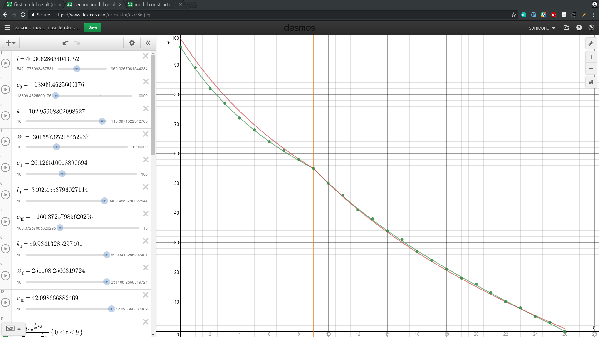
I’ll now look at the two configurations that I obtained and plot them. The red line shows the worst configuration, and the green line shows the best configuration.
As you can see in second_model_code_result rounded predictions of the best configuration exactly match the given data.
Conclusion of Model 2
\begin{equation}
\begin{cases}
v = \frac{λ e\frac{λ{m} c_3}}{e\frac{λ{m} t} - ke\frac{λ{m}c_3}}, & t ∈ [0, 9]
v = \frac{\sqrt{4kW - λ^2}tan(\frac{\sqrt{4kW-λ^2}}{2m}(c_4 - t)) - λ}{2k}, & t ∈ [9, 26] \
λ = 40.30628634043052 \
c_3 = -13809.4625600176 \
k = 102.95908302098627 \
W = 301557.65216452937 \
c_4 = 26.126510013890694 \
\end{cases}
\end{equation}
As you can see the value of
Assessment of the improvement obtained
Prediction
Based on the models I predict that the aeroplane stopped in
Comparing the models
| Time | Predicted | Predicted | Observed | Better |
| Speed | Speed | Speed | Model | |
| (1st Model) | (2nd Model) | |||
|---|---|---|---|---|
| 0.0 | 96.0 | 96.0000000000054 | 96 | 1st |
| 1.0 | 88.65671641791045 | 88.66582512227822 | 89 | 2nd |
| 2.0 | 82.35701906412478 | 82.37077686914407 | 82 | 1st |
| 3.0 | 76.89320388349515 | 76.90862555559508 | 77 | 2nd |
| 4.0 | 72.1092564491654 | 72.12432763292139 | 72 | 1st |
| 5.0 | 67.88571428571429 | 67.89907302369585 | 68 | 2nd |
| 6.0 | 64.12955465587045 | 64.14028474770049 | 64 | 1st |
| 7.0 | 60.767263427109974 | 60.77475738769026 | 61 | 2nd |
| 8.0 | 57.739975698663415 | 57.743842139329196 | 58 | 2nd |
| 9.0 | 54.99999999999999 | 55.00000000000179 | 55 | 1st |
| 10.0 | 50.10816658852111 | 50.10157524003789 | 50 | 2nd |
| 11.0 | 45.622063036212374 | 45.60871998373162 | 46 | 2nd |
| 12.0 | 41.475988862696376 | 41.45588373779139 | 41 | 2nd |
| 13.0 | 37.61659930730753 | 37.5898231332195 | 38 | 1st |
| 14.0 | 34.00002062308155 | 33.96673336319917 | 34 | 1st |
| 15.0 | 30.589724513917773 | 30.550133354391157 | 31 | 1st |
| 16.0 | 27.35493651754378 | 27.309281417030515 | 27 | 2nd |
| 17.0 | 24.269426053394415 | 24.217970303658813 | 24 | 2nd |
| 18.0 | 21.3105731783461 | 21.253597490201017 | 21 | 2nd |
| 19.0 | 18.45863841578133 | 18.396437545757497 | 18 | 2nd |
| 20.0 | 15.696183121094782 | 15.629064386691416 | 16 | 1st |
| 21.0 | 13.00760227741885 | 12.935885534732083 | 13 | 1st |
| 22.0 | 10.378741615250261 | 10.30276043083657 | 10 | 2nd |
| 23.0 | 7.796577949697343 | 7.716681813438704 | 8 | 1st |
| 24.0 | 5.248946558956161 | 5.165504072768728 | 5 | 2nd |
| 25.0 | 2.7243028986249413 | 2.6377059483218517 | 3 | 1st |
| 26.0 | 0.2115083630415522 | 0.12217734574065967 | 0 | 2nd |
| Model | Maximum Error | Average Error | Root mean square | Num. of better |
| predictions | ||||
|---|---|---|---|---|
| 1st | 0.47598886269637575 | 0.23822424753496707 | 0.2776875104911393 | 12 |
| 2nd | 0.4558837377913889 | 0.23458170693637476 | 0.27311676642511934 | 15 |
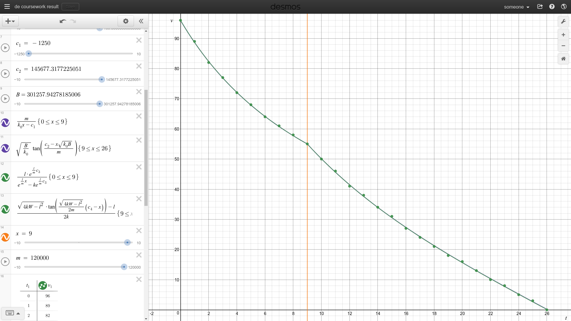
Here is a graph of both of the models. The purple line is the first model and the green line is the second one.
The curves are so close to each other that at this scale you can’t even see the difference. The second model gave more accurate predictions, but the increase in accuracy is very small and the increases in complexity and computation time are significant.
