willb / cml_churn_demo_mlops

Churn Prediction Prototype

This project is a Cloudera Machine Learning (CML) Applied Machine Learning Project Prototype. It has all the code and data needed to deploy an end-to-end machine learning project in a running CML instance.

Project Overview

This project builds the telco churn with model interpretability project discussed in more detail this blog post. The initial idea and code comes from the FFL Interpretability report which is now freely available and you can read the full report here

The goal is to build a classifier model using Logistic Regression to predict the churn probability for a group of customers from a telecoms company. On top that, the model can then be interpreted using LIME. Both the Logistic Regression and LIME models are then deployed using CML's real-time model deployment capability and finally a basic flask based web application is deployed that will let you interact with the real-time model to see which factors in the data have the most influence on the churn probability.

By following the notebooks in this project, you will understand how to perform similar classification tasks on CML as well as how to use the platform's major features to your advantage. These features include streamlined model experimentation, point-and-click model deployment, and ML app hosting.

We will focus our attention on working within CML, using all it has to offer, while glossing over the details that are simply standard data science. We trust that you are familiar with typical data science workflows and do not need detailed explanations of the code. Notes that are specific to CML will be emphasized in block quotes.

Initialize the Project

There are a couple of steps needed at the start to configure the Project and Workspace settings so each step will run sucessfully. You must run the project bootstrap before running other steps. If you just want to launch the model interpretability application without going through each step manually, then you can also deploy the complete project.

Project bootstrap

Open the file 0_bootstrap.py in a normal workbench python3 session. You only need a 1 vCPU / 2 GiB instance. Once the session is loaded, click Run > Run All Lines. This will file will create an Environment Variable for the project called STORAGE, which is the root of default file storage location for the Hive Metastore in the DataLake (e.g. s3a://my-default-bucket). It will also upload the data used in the project to $STORAGE/datalake/data/churn/. The original file comes as part of this git repo in the raw folder.

Deploy the Complete Project

If you just wish build the project artifacts without going through each step manually, run the 8_build_projet.py file in a python3 session. Again a 1 vCPU / 2 GiB instance will be suffient. This script will:

• run the bootstrap
• then create the Hive Table and import the data
• deploy the model
• update the application files to use this new model
• deploy the application
• run the model drift simulation Once the script has completed you will see the new model and application are now available in the project.

Project Build

If you want go through each of the steps manually to build and understand how the project works, follow the steps below. There is a lot more detail and explanation/comments in each of the files/notebooks so its worth looking into those. Follow the steps below and you will end up with a running application.

0 Bootstrap

Just to reiterate that you have run the bootstrap for this project before anything else. So make sure you run step 0 first.

Open the file 0_bootstrap.py in a normal workbench python3 session. You only need a 1 CPU / 2 GB instance. Then Run > Run All Lines

1 Ingest Data

This script will read in the data csv from the file uploaded to the object store (s3/adls) setup during the bootstrap and create a managed table in Hive. This is all done using Spark.

Open 1_data_ingest.py in a Workbench session: python3, 1 CPU, 2 GB. Run the file.

2 Explore Data

This is a Jupyter Notebook that does some basic data exploration and visualistaion. It is to show how this would be part of the data science workflow.

Open a Jupyter Notebook session (rather than a work bench): python3, 1 CPU, 2 GB and open the 2_data_exploration.ipynb file.

At the top of the page click Cells > Run All.

3 Model Building

This is also a Jupyter Notebook to show the process of selecting and building the model to predict churn. It also shows more details on how the LIME model is created and a bit more on what LIME is actually doing.

Open a Jupyter Notebook session (rather than a work bench): python3, 1 CPU, 2 GB and open the 3_model_building.ipynb file.

At the top of the page click Cells > Run All.

4 Model Training

A model pre-trained is saved with the repo has been and placed in the models directory. If you want to retrain the model, open the 4_train_models.py file in a workbench session: python3 1 vCPU, 2 GiB and run the file. The newly model will be saved in the models directory named telco_linear.

There are 2 other ways of running the model training process

1. Jobs

The Jobs feature allows for adhoc, recurring and depend jobs to run specific scripts. To run this model training process as a job, create a new job by going to the Project window and clicking Jobs > New Job and entering the following settings:

• Name : Train Mdoel
• Script : 4_train_models.py
• Arguments : Leave blank
• Kernel : Python 3
• Schedule : Manual
• Engine Profile : 1 vCPU / 2 GiB The rest can be left as is. Once the job has been created, click Run to start a manual run for that job.

2. Experiments

The other option is running an Experiment. Experiments run immediately and are used for testing different parameters in a model training process. In this instance it would be use for hyperparameter optimisation. To run an experiment, from the Project window click Experiments > Run Experiment with the following settings.

• Script : 4_train_models.py
• Arguments : 5 lbfgs 100 _(these the cv, solver and max_iter parameters to be passed to LogisticRegressionCV() function)
• Kernel : Python 3
• Engine Profile : 1 vCPU / 2 GiB

Click Start Run and the expriment will be sheduled to build and run. Once the Run is completed you can view the outputs that are tracked with the experiment using the cdsw.track_metrics function. It's worth reading through the code to get a sense of what all is going on.

5 Serve Model

The Models is used top deploy a machine learning model into production for real-time prediction. To deploy the model trailed in the previous step, from to the Project page, click Models > New Model and create a new model with the following details:

• Name: Explainer
• Description: Explain customer churn prediction
• File: 5_model_serve_explainer.py
• Function: explain
• Input:

{
	"StreamingTV": "No",
	"MonthlyCharges": 70.35,
	"PhoneService": "No",
	"PaperlessBilling": "No",
	"Partner": "No",
	"OnlineBackup": "No",
	"gender": "Female",
	"Contract": "Month-to-month",
	"TotalCharges": 1397.475,
	"StreamingMovies": "No",
	"DeviceProtection": "No",
	"PaymentMethod": "Bank transfer (automatic)",
	"tenure": 29,
	"Dependents": "No",
	"OnlineSecurity": "No",
	"MultipleLines": "No",
	"InternetService": "DSL",
	"SeniorCitizen": "No",
	"TechSupport": "No"
}

• Kernel: Python 3
• Engine Profile: 1vCPU / 2 GiB Memory

Leave the rest unchanged. Click Deploy Model and the model will go through the build process and deploy a REST endpoint. Once the model is deployed, you can test it is working from the model Model Overview page.

Note: This is important

Once the model is deployed, you must disable the additional model authentication feature. In the model settings page, untick Enable Authentication.

6 Deploy Application

The next step is to deploy the Flask application. The Applications feature is still quite new for CML. For this project it is used to deploy a web based application that interacts with the underlying model created in the previous step.

Note: This next step is important

In the deployed model from step 5, go to Model > Settings and make a note (i.e. copy) the "Access Key". It will look something like this (ie. mukd9sit7tacnfq2phhn3whc4unq1f38)

From the Project level click on "Open Workbench" (note you don't actually have to Launch a session) in order to edit a file. Select the flask/single_view.html file and paste the Access Key in at line 19.

const accessKey = "mp3ebluylxh4yn5h9xurh1r0430y76ca";

Save the file (if it has not auto saved already) and go back to the Project.

From the Go to the Applications section and select "New Application" with the following:

• Name: Churn Analysis App
• Subdomain: churn-app (note: this needs to be unique, so if you've done this before, pick a more random subdomain name)
• Script: 6_application.py
• Kernel: Python 3
• Engine Profile: 1vCPU / 2 GiB Memory

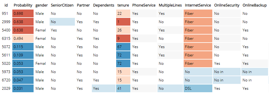
After the Application deploys, click on the blue-arrow next to the name. The initial view is a table of randomly selected from the dataset. This shows a global view of which features are most important for the predictor model. The reds show incresed importance for preditcting a cusomter that will churn and the blues for for customers that will not.

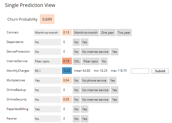
Clicking on any single row will show a "local" interpreted model for that particular data point instance. Here you can see how adjusting any one of the features will change the instance's churn prediction.

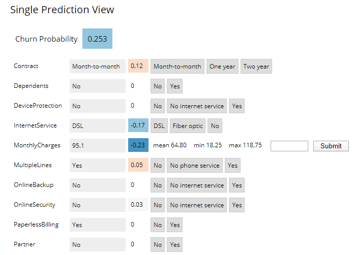
Changing the InternetService to DSL lowers the probablity of churn. Note: this does not mean that changing the Internet Service to DSL cause the probability to go down, this is just what the model would predict for a customer with those data points

7 Model Operations

The final step is the model operations which consists of Model Metrics and Model Governance

Model Governance is setup in the 0_bootstrap.py script, which writes out the lineage.yml file at the start of the project. For the Model Metrics open a workbench session (1 vCPU / 2 GiB) and open the 7a_ml_ops_simulation.py file. You need to set the model_id number from the model created in step 5 on line 113. The model number is on the model's main page.

model_id = "95"

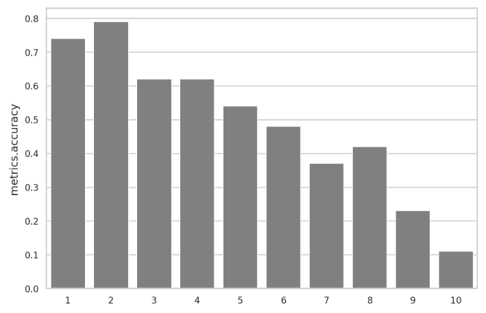
From there, run the file. This goes through a process of simulating an model that drifts over over 1000 calls to the model. The file contains comments with details of how this is done.

In the next step you can interact and display the model metrics. Open a workbench session (1 vCPU / 2 GiB) and open and run the 7b_ml_ops_visual.py file. Again you need to set the model_id number from the model created in step 5 on line 53. The model number is on the model's main page.