USF-IMARS / cr-metrics

Condition Report metrics to inform National Marine Sanctuaries

cr-metrics

Condition Report metrics to inform on National Marine Sanctuaries status using interactive infographic approach to displaying habitat-based elements that link to time series data. Proposed by Jenn Brown (2016).

Creation

Given a vector illustration of habitat scenes with different elements (eg pelagic: whales, fish, etc), running the following R code will generate the website for pulling up timeseries plots by clicking on the elements:

# create pages
source('functions.R') # clear_site()
create_site()

Technology Overview

The core functionality of this interactive infographic is to link graphical elements to interactive plots of time series or maps:

• Ecosystem elements should be in the form of scalable vector graphics (*.svg), the most popular vector format (vs raster images) for illustration and animation on the web.

• Interactive plots are easily generated with the cross-platform statistical programming language R and the many packages utilizing the htmlwidgets framework for porting JavaScript data visualization libraries to R functions that feed in the data. Check out the htmlwidgets showcase for compelling examples. The data pages with these htmlwidgets embedded are generated using the Rmarkdown package, which weaves in simple formatted text with evaluated chunks of R code to render in any desired output format (html, doc, pdf...). I strongly encourage you to watch the 1 minute video What is R Markdown? on Vimeo. You can see the R code that generates these pages from the data/csv_indicators.csv at functions.R.

To link the svg elements with the indicator plots, the powerful d3 JavaScript library is used to read in the data/svg_elements.csv and apply links to the elements. See code in _svg.Rmd.

Files

Here's an overview of all the files as a tree in alphabetic order, except for habitat Rmarkdown files to show similarity.

$ tree -L 2
.
├── README.md                # this README with instructions
├── _footer.html             # website header
├── _header.html             # website footer
├── _site.yml                # site menu
├── _svg.Rmd                 # child Rmarkdown for habitats
├── coral-reef.Rmd           # habitat Rmarkdown
├── kelp-forest.Rmd          # habitat Rmarkdown
├── pelagic.Rmd              # habitat Rmarkdown
├── cr-metrics.Rproj         # R project file (optional)
├── data/                    # data folder
│   ├── csv_indicators.csv   # - table of timeseries csv
│   └── svg_elements.csv     # - table of svg elements
├── docs/                    # website folder, gets regenerated
├── functions.R              # core functions to creat website
├── img/                     # images for README
├── index.Rmd                # home page of website
├── libs/                    # libraries folder
│   ├── d3-dsv.v1.min.js     # - JavaScript to read csv
│   ├── d3.v3.min.js         # - JavaScript to manipulate svg
│   └── styles.css           # - minor styling with CSS
├── svg/                     # svg folder
│   ├── coral-reef.svg       # - habitat svg
│   ├── kelp-forest.svg      # - habitat svg
│   └── pelagic.svg          # - habitat svg
└── svg_prep/                # svg prep files (deletable)

Process

Besides the habitat illustration as a scalable vector graphics file (eg pelagics.svg), the create_site() function relies on two tables in comma-seperated value (data/*.csv) format:

• svg_elements.csv: identifies the elements in the svg habitat scene(s)
• csv_indicators.csv: provides the ERDDAP URL to the timeseries data and other parameters to describe the timeseries plots and match to the svg element

The website content is output to the docs/ folder, providing an interactive user experience with only basic web files (*.html, *.js, *.css) that any web server can host.

You can see the files for this site hosted on Github here:

• https://github.com/marinebon/cr-metrics

Please visit Help & Documentation for MBON - Applications - Interactive Infographics for more background.

Here are detailed steps to prep the necessary files (svg scenes, csv tables of elements and indicators)...

1. Download and unzip the template site here:

• https://github.com/marinebon/cr-metrics/archive/master.zip

1. Edit the vector graphics file of the habitat scene with elements using the free Inkscape program that natively uses scalable vector graphics (*.svg) format:

   • remove text labels

   • add ID to element or group of elements:

     

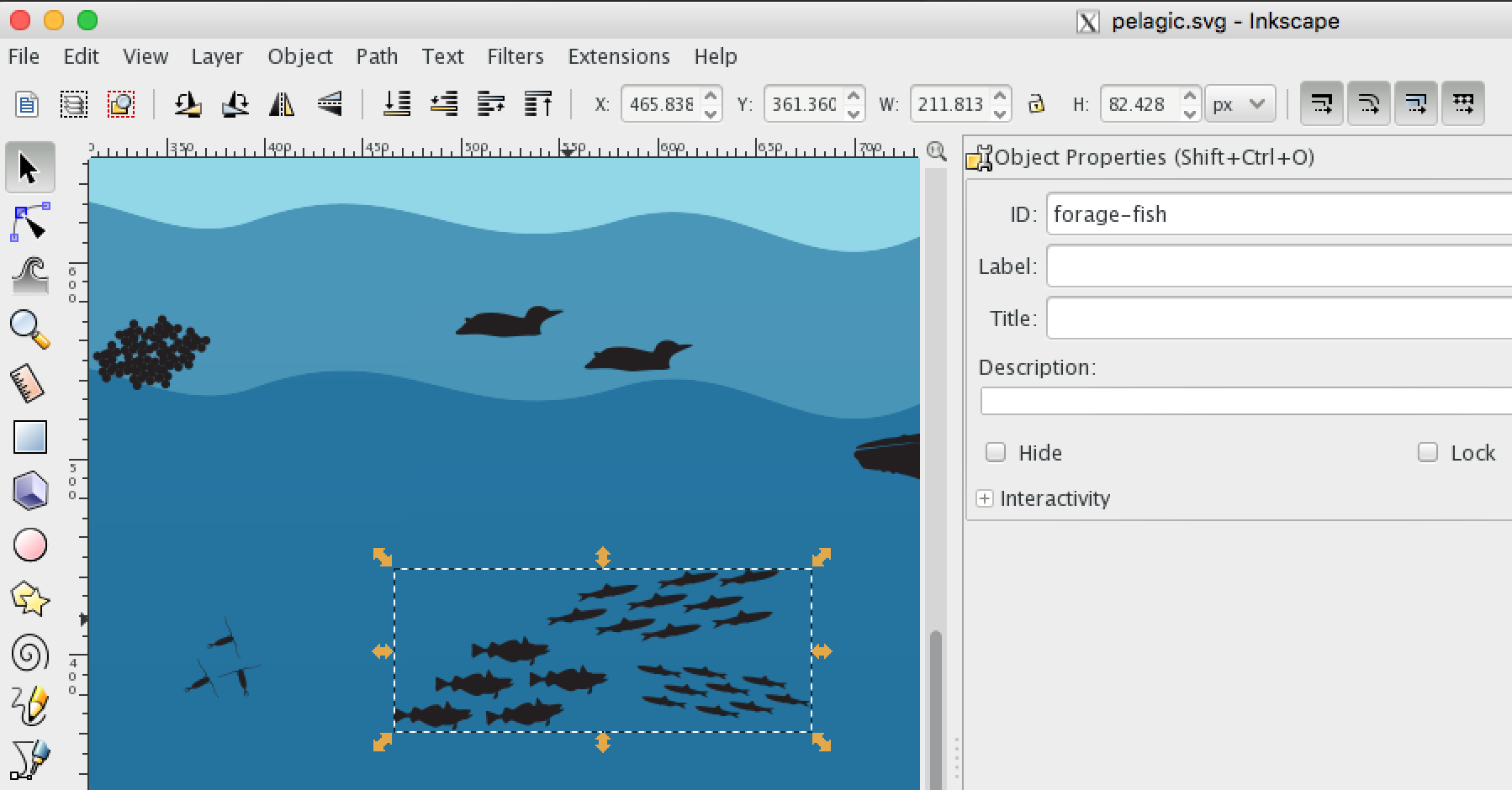
   • save to folder svg/*.svg as "Plain SVG" (such as svg/pelagic.svg)

2. Add rows to the svg/elements.csv:

   habitat	id	status_path	status_color	status_text	link_path	link	link_title
   pelagic	whales	path#whales	red	decreasing	path#whales	./pages/pinnipeds.html	Whales
   pelagic	forage-fish	g#forage-fish path	green	increasing	g#forage-fish	./pages/pinnipeds.html	Forage Fish
   kelp-forest	otters	path#otters	purple	stable	path#otter	./pages/pinnipeds.html	Sea Otters

   • habitat: the unique name to filter for elements of this habitat scene
   • id: unique element identifier
   • status_path: the SVG path, either path#element (eg path#whales) for single element, or g#element path for grouped elements (eg g#forage-fish path)
   • status_color: the color of the element reflecting the status
   • status_text: the text of the element reflecting the status that appears on hover
   • link_path: the SVG path, either path#element (eg path#whales) for single element, or g#element for grouped elements (eg g#forage-fish)
   • link: the hyperlink to the page of corresponding data (usually timeseries)
   • link_title: the title that shows at the top of the modal popup window containing the page when the element is clicked

3. Add / edit the data/csv_indicators.csv with the following key fields, originally drawn from the site IEA - California Current:

   • indicator: name of indicator, which will become the timeseries plot's title
   • y_label: label on the y-axis describing the value measured over time
   • csv_url: the link to the ERDDAP data in CSV format, extractable from the ERDDAP image URL

4. Create the site by running the following R code:

source('functions.R') create_site()

    - Be sure that your current working directory is in the `cr-metrics/` root folder (eg with `setwd()` in R).

    The website gets built into the `docs/` folder.

5. Push to website. This repository uses Github Pages:

    - code: https://github.com/marinebon/cr-metrics

    - site: https://marinebon.github.io/cr-metrics

## TODO

- Seperate into R package infographiq, and instances for FKNMS, MBNMS, etc.

- Populate California example, using available ERDDAP-connected timeseries from [IEA - California Current](https://www.integratedecosystemassessment.noaa.gov//regions/california-current-region/index.html)

- Populate Florida Keys NMS, working in particular with people at FKNMS (Mike Buchman, Steve Gittings) and FL MBON (Megan Hepner)