YOLOv5 (6.0/6.1) brief summary
WZMIAOMIAO opened this issue · comments

Content
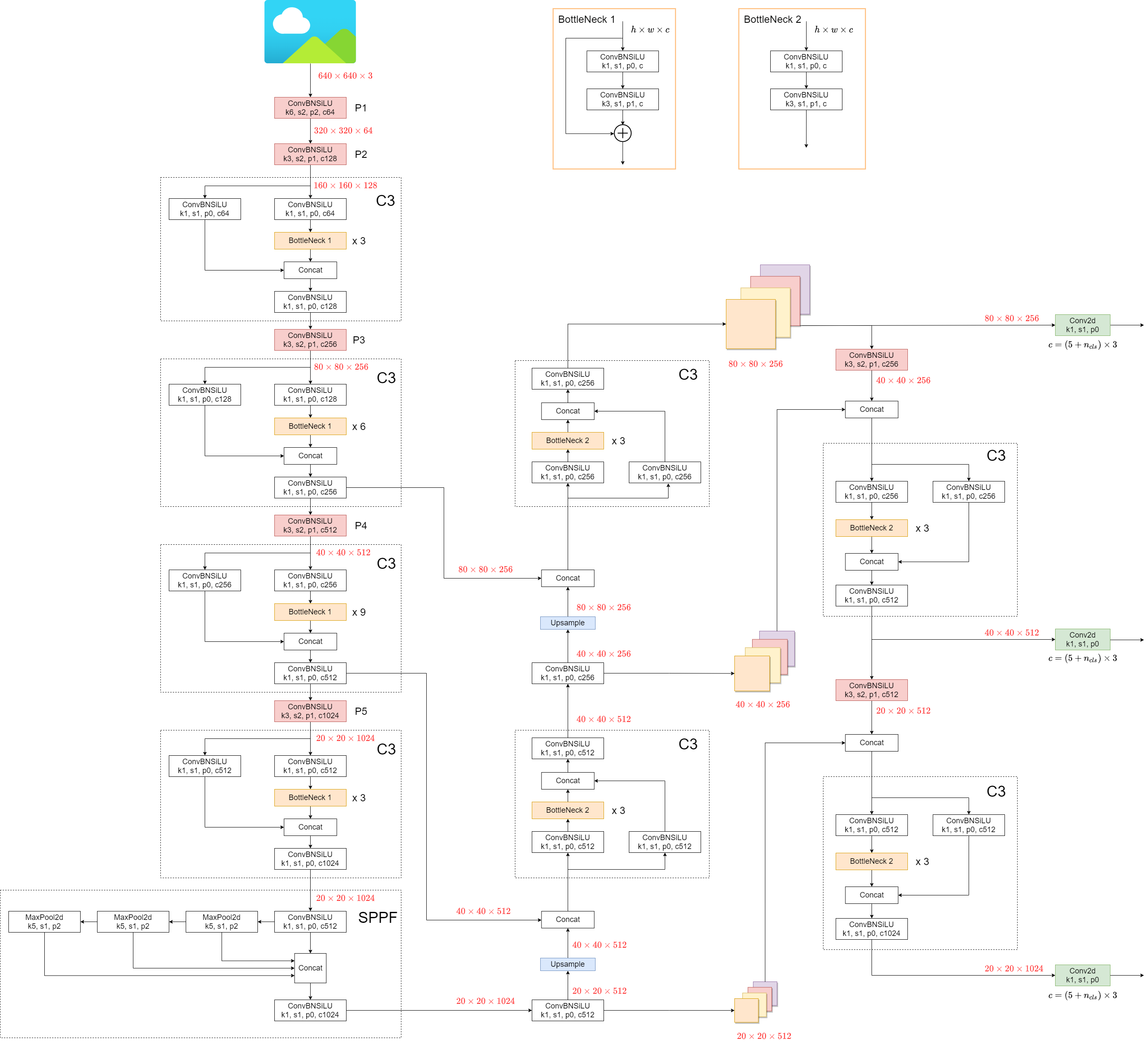
1. Model Structure
YOLOv5 (v6.0/6.1) consists of:
- Backbone:
New CSP-Darknet53 - Neck:
SPPF,New CSP-PAN - Head:
YOLOv3 Head
Model structure (yolov5l.yaml):
Some minor changes compared to previous versions:
- Replace the
Focusstructure with6x6 Conv2d(more efficient, refer #4825) - Replace the
SPPstructure withSPPF(more than double the speed)
test code
import time
import torch
import torch.nn as nn


class SPP(nn.Module):
    def __init__(self):
        super().__init__()
        self.maxpool1 = nn.MaxPool2d(5, 1, padding=2)
        self.maxpool2 = nn.MaxPool2d(9, 1, padding=4)
        self.maxpool3 = nn.MaxPool2d(13, 1, padding=6)

    def forward(self, x):
        o1 = self.maxpool1(x)
        o2 = self.maxpool2(x)
        o3 = self.maxpool3(x)
        return torch.cat([x, o1, o2, o3], dim=1)


class SPPF(nn.Module):
    def __init__(self):
        super().__init__()
        self.maxpool = nn.MaxPool2d(5, 1, padding=2)

    def forward(self, x):
        o1 = self.maxpool(x)
        o2 = self.maxpool(o1)
        o3 = self.maxpool(o2)
        return torch.cat([x, o1, o2, o3], dim=1)


def main():
    input_tensor = torch.rand(8, 32, 16, 16)
    spp = SPP()
    sppf = SPPF()
    output1 = spp(input_tensor)
    output2 = sppf(input_tensor)

    print(torch.equal(output1, output2))

    t_start = time.time()
    for _ in range(100):
        spp(input_tensor)
    print(f"spp time: {time.time() - t_start}")

    t_start = time.time()
    for _ in range(100):
        sppf(input_tensor)
    print(f"sppf time: {time.time() - t_start}")


if __name__ == '__main__':
    main()
result:
True
spp time: 0.5373051166534424
sppf time: 0.20780706405639648
2. Data Augmentation
- Mosaic

- Copy paste

- Random affine(Rotation, Scale, Translation and Shear)

- MixUp

- Albumentations
- Augment HSV(Hue, Saturation, Value)

- Random horizontal flip

3. Training Strategies
- Multi-scale training(0.5~1.5x)
- AutoAnchor(For training custom data)
- Warmup and Cosine LR scheduler
- EMA(Exponential Moving Average)
- Mixed precision
- Evolve hyper-parameters
4. Others
4.1 Compute Losses
The YOLOv5 loss consists of three parts:
- Classes loss(BCE loss)
- Objectness loss(BCE loss)
- Location loss(CIoU loss)
4.2 Balance Losses
The objectness losses of the three prediction layers(P3, P4, P5) are weighted differently. The balance weights are [4.0, 1.0, 0.4] respectively.
4.3 Eliminate Grid Sensitivity
In YOLOv2 and YOLOv3, the formula for calculating the predicted target information is:

In YOLOv5, the formula is:
Compare the center point offset before and after scaling. The center point offset range is adjusted from (0, 1) to (-0.5, 1.5).
Therefore, offset can easily get 0 or 1.

Compare the height and width scaling ratio(relative to anchor) before and after adjustment. The original yolo/darknet box equations have a serious flaw. Width and Height are completely unbounded as they are simply out=exp(in), which is dangerous, as it can lead to runaway gradients, instabilities, NaN losses and ultimately a complete loss of training. refer this issue

4.4 Build Targets
Match positive samples:
- Calculate the aspect ratio of GT and Anchor Templates

- Assign the successfully matched Anchor Templates to the corresponding cells

- Because the center point offset range is adjusted from (0, 1) to (-0.5, 1.5). GT Box can be assigned to more anchors.

Environments
YOLOv5 may be run in any of the following up-to-date verified environments (with all dependencies including CUDA/CUDNN, Python and PyTorch preinstalled):
- Notebooks with free GPU:
- Google Cloud Deep Learning VM. See GCP Quickstart Guide
- Amazon Deep Learning AMI. See AWS Quickstart Guide
- Docker Image. See Docker Quickstart Guide


Status
![]()
If this badge is green, all YOLOv5 GitHub Actions Continuous Integration (CI) tests are currently passing. CI tests verify correct operation of YOLOv5 training, validation, inference, export and benchmarks on MacOS, Windows, and Ubuntu every 24 hours and on every commit.
@glenn-jocher hi, today I briefly summarized yolov5(v6.0). Please help to see if there are any problems or put forward better suggestions. Some schematic diagrams or contents will be added later. Thank you for your great work.

hi, 'prediction layers(P3, P4, P5) are weighted differently', how do I find it in the code, and further, modify it?
@WZMIAOMIAO thx!

@WZMIAOMIAO awesome summary, nice work!
@zlj-ky yes the balancing parameters are there, we tuned these manually on COCO. The idea is to balance losses from each layer (just like we balance losses across loss components (box, obj, class)). The reason I didn't turn these into learnable weights is that as absolute values the gradient would always want to drag them to zero to minimize the loss. I suppose we could constantly normalize them so they all sum to 1 to avoid this effect. Might be an interesting experiment, and this might help the balancing adapt better to different datasets and image sizes etc.
@glenn-jocher Could we add this brief summary to the document?
@WZMIAOMIAO yes maybe it's a good idea to document this somewhere. Which document do you mean though?
@glenn-jocher I think it could be added to the Tutorials. What do you think?
@WZMIAOMIAO all done in #7146! Thank you for your contributions to YOLOv5 🚀 and Vision AI ⭐
@HERIUN built_targets() implements an anchor-label assignment strategy so we can calculate the losses between assigned anchor-label pairs.

@glenn-jocher what's the adjustment strategy for the balancing parameters?How to change them to learnable weights?
@WZMIAOMIAO awesome summary, nice work!
@zlj-ky yes the balancing parameters are there, we tuned these manually on COCO. The idea is to balance losses from each layer (just like we balance losses across loss components (box, obj, class)). The reason I didn't turn these into learnable weights is that as absolute values the gradient would always want to drag them to zero to minimize the loss. I suppose we could constantly normalize them so they all sum to 1 to avoid this effect. Might be an interesting experiment, and this might help the balancing adapt better to different datasets and image sizes etc.
@glenn-jocher what's the adjustment strategy for the balancing parameters?How to change them to learnable weights?
@xinxin342 the balance params are here, you'd have to convert them to nn.Parameter types assigned to an existing class and set their compute grad to True:
Line 112 in c9a3b14
@xinxin342 the balance params are here, you'd have to convert them to nn.Parameter types assigned to an existing class and set their compute grad to True:
Line 112 in c9a3b14
@glenn-jocher
I try to convert the weight to a learnable parameter like this(Limited by my limited experience)

However, this parameter was not updated during training, I don't know why or how to revise my method. Can you teach me, even though it's a very simple question
@zlj-ky that seems like a good approach, but you might need to place self.w inside the model so it's affected by model.train(), model.eval(), etc. You can just place it inside models.yolo.Detect and then access it like this. (Note your code is out of date):
class ComputeLoss:
    sort_obj_iou = False

    def __init__(self, model, autobalance=False):
        device = next(model.parameters()).device  # get model device
        h = model.hyp  # hyperparameters

        # Define criteria
        BCEcls = nn.BCEWithLogitsLoss(pos_weight=torch.tensor([h['cls_pw']], device=device))
        BCEobj = nn.BCEWithLogitsLoss(pos_weight=torch.tensor([h['obj_pw']], device=device))

        # Class label smoothing https://arxiv.org/pdf/1902.04103.pdf eqn 3
        self.cp, self.cn = smooth_BCE(eps=h.get('label_smoothing', 0.0))  # positive, negative BCE targets

        # Focal loss
        g = h['fl_gamma']  # focal loss gamma
        if g > 0:
            BCEcls, BCEobj = FocalLoss(BCEcls, g), FocalLoss(BCEobj, g)

        m = de_parallel(model).model[-1]  # Detect() module
        self.balance = {3: [4.0, 1.0, 0.4]}.get(m.nl, [4.0, 1.0, 0.25, 0.06, 0.02])  # P3-P7
        self.ssi = list(m.stride).index(16) if autobalance else 0  # stride 16 index
        self.BCEcls, self.BCEobj, self.gr, self.hyp, self.autobalance = BCEcls, BCEobj, 1.0, h, autobalance
        self.na = m.na  # number of anchors
        self.nc = m.nc  # number of classes
        self.nl = m.nl  # number of layers
        self.anchors = m.anchors
        self.w = m.w  # <------------------------ NEW CODE
        self.device = device
This might or might not work as I don't know if this will create a copy or access the Detect parameter.
Even if you get this to work though It's not clear that these are learnable parameters as I'm not sure if they can be correlated to the gradient directly, i.e. the optimizer seeks to reduce loss, so the rebalance may just weigh higher the lower loss components to reduce loss, which may not have the desired effect.
The same concept applies to anchors, which don't seem learnable either during training.
@glenn-jocher Thank you for sharing your views on this matter and for your patient guidance. I will try it latter.

@HERIUN built_targets() implements an anchor-label assignment strategy so we can calculate the losses between assigned anchor-label pairs.


I can't match from code to explaining figure...
where c_x, c_y are in code??
and during calculating pwh in code.. why anchor[i] is p_w,h ??
@HERIUN built_targets() implements an anchor-label assignment strategy so we can calculate the losses between assigned anchor-label pairs.
I can't match from code to explaining figure... where c_x, c_y are in code?? and during calculating pwh in code.. why anchor[i] is p_w,h ??
This figure shows the coordinate calculation formula of yolov2 and v3, not v5. For coordinate calculation, please refer to the following code:
Lines 66 to 72 in 7926afc
If there is anything unclear, I suggest you check each variable through debug

For the doubts about ‘grid-0.5’, I see many such problems, eg #6252, #471...
Compared with the previous code(y[..., 0:2] *2 - 0.5 + grid), I found that the step of subtracting 0.5 was put into the calculation of grid;
I don't quite understand why? Doesn't the mesh grid(i,j) exactly represent the top left corner vertex of the mesh in row I and column J? After subtracting 0.5, the center will move to the center of the upper left grid(i-1, J-1).
We look forward to your reply
@isJunCheng grid computation now embeds offsets (after #7262) to reduce FLOPs in detect.py and simplify export models. The change has no mathematical implications, the result is exactly the same as before.
@isJunCheng grid computation now embeds offsets (after #7262) to reduce FLOPs in detect.py and simplify export models. The change has no mathematical implications, the result is exactly the same as before.
thank you for your reply.
I haven't found an article that can make me understand. Can you explain it? After subtracting 0.5, where is the center of the anchor? The upper left corner of the (I, J) grid or the center of the (i-1, J-1) grid.
I want to know where the anchor center is.

@zlj-ky that seems like a good approach, but you might need to place self.w inside the model so it's affected by model.train(), model.eval(), etc. You can just place it inside models.yolo.Detect and then access it like this. (Note your code is out of date):
class ComputeLoss:
    sort_obj_iou = False

    def __init__(self, model, autobalance=False):
        device = next(model.parameters()).device  # get model device
        h = model.hyp  # hyperparameters

        # Define criteria
        BCEcls = nn.BCEWithLogitsLoss(pos_weight=torch.tensor([h['cls_pw']], device=device))
        BCEobj = nn.BCEWithLogitsLoss(pos_weight=torch.tensor([h['obj_pw']], device=device))

        # Class label smoothing https://arxiv.org/pdf/1902.04103.pdf eqn 3
        self.cp, self.cn = smooth_BCE(eps=h.get('label_smoothing', 0.0))  # positive, negative BCE targets

        # Focal loss
        g = h['fl_gamma']  # focal loss gamma
        if g > 0:
            BCEcls, BCEobj = FocalLoss(BCEcls, g), FocalLoss(BCEobj, g)

        m = de_parallel(model).model[-1]  # Detect() module
        self.balance = {3: [4.0, 1.0, 0.4]}.get(m.nl, [4.0, 1.0, 0.25, 0.06, 0.02])  # P3-P7
        self.ssi = list(m.stride).index(16) if autobalance else 0  # stride 16 index
        self.BCEcls, self.BCEobj, self.gr, self.hyp, self.autobalance = BCEcls, BCEobj, 1.0, h, autobalance
        self.na = m.na  # number of anchors
        self.nc = m.nc  # number of classes
        self.nl = m.nl  # number of layers
        self.anchors = m.anchors
        self.w = m.w  # <------------------------ NEW CODE
        self.device = device
This might or might not work as I don't know if this will create a copy or access the Detect parameter.
Even if you get this to work though It's not clear that these are learnable parameters as I'm not sure if they can be correlated to the gradient directly, i.e. the optimizer seeks to reduce loss, so the rebalance may just weigh higher the lower loss components to reduce loss, which may not have the desired effect.
The same concept applies to anchors, which don't seem learnable either during training.
Hey @glenn-jocher ,
I've been dealing with the issue of balancing losses in another project of mine. I feel that adding multiple losses and passing that loss to the Adam (or AdamW etc.) optimizer will not be able to optimize well. (Since the learning rate is adjusted for each parameter, Adam can't figure out which loss component has bigger effect. )
for example:
loss1 = BCEWithLogitLoss(pred[0:2]) , target[0:2]) loss2 = MSE(pred[2:4]), target[2:4]) loss = loss1 + loss2 loss.backward() optimizer.step()
More reference for the same : https://discuss.pytorch.org/t/how-are-optimizer-step-and-loss-backward-related/7350/14
The stackoverflow page the above post mentions : https://stackoverflow.com/questions/46774641/what-does-the-parameter-retain-graph-mean-in-the-variables-backward-method
There's something called MTAdam for the same.
Are these considerations needed if I'm training on a dataset with just one tiny object per image and only one class in the dataset [without any pretraining]? (Assuming that the difference in losses would be massive, no-object loss would dominate in this case since we only have one object per image and the rest of the cells should predict no-object).
@AnkushMalaker you can find the objectness loss hyps here:
yolov5/data/hyps/hyp.scratch-low.yaml
Lines 16 to 17 in d059d1d
In terms of balancing losses this has nothing to do with the amount of labels an image has, this balancing is across output layers P3-P6

@glenn-jocher Dear, I still don't quite understand what criteria are taken into account to define these weights: P3 (4.0), P4 (1.0) and P5 (0.4)?
That is, how were these weights arrived at and what is the influence of these weights on the detection, for example, of small objects?
@glenn-jocher Another question I have is about the number of neurons and hidden layers in the network.
How do I get this information?
@carlossantos-iffar the purpose is the balance the loss contributions from the difference outputs.
@carlossantos-iffar the purpose is the balance the loss contributions from the difference outputs.
Perfect! But my question is how did you arrive at these weight values? 4.0, 1.0 and 0.4?
@carlossantos-iffar from empirical observations of actual losses on default COCO trainings
@carlossantos-iffar from empirical observations of actual losses on default COCO trainings
Thanks!

I would like to ask how can I change this function if my output layer has four layers

The Balance Losses is objectness loss?
Can you elaborate on the loss function?
thank you.
@glenn-jocher Sorry to ping you again on this thread, since there are comments discussing the summary/loss, thought this is the appropriate place. I saw in this comment that you switched to BCE loss for class classification instead of CE loss due to some epxeriments in YOLOv3. I tried to look for issues explaining why the change in YOLOv3 repository but couldn't find a lead. Could you elaborate or point me to where I could understand the reasoning?
In my understanding, currently we the class classification as a multi label problem. In a situation where we only have two classes that are binary (Say, class1: Fluffy cat. Class2: Slim cat) where we can never have both of them active at the same time, I should instead use CE loss, right?

@AnkushMalaker you can find the objectness loss hyps here:
yolov5/data/hyps/hyp.scratch-low.yaml
Lines 16 to 17 in d059d1d
In terms of balancing losses this has nothing to do with the amount of labels an image has, this balancing is across output layers P3-P6
I do not understand why the positive and negative objectness values have the same weight. When I try it in my custom implementations the non-object values overwhelm the object values and it only works when I weight them separately and reduce the impact of non-objectness score as in the original YOLO paper that had separated objectnes and non-objectness scores.
Is there something that I am missing. Are you balancing them in another way?
@carlossantos-iffar the purpose is the balance the loss contributions from the difference outputs.
Perfect! But my question is how did you arrive at these weight values? 4.0, 1.0 and 0.4?
The way I understand it is that the last detection layer has fewer output neurons than the higher resolution map. Since when we average the higher resolution map will be divided with a larger number it's influence is reduces. Hence, multiplying it with a larger number balances this. I usually use the factor of resolution as balancing weight. Hence, I use 1 for the lowes dim map, 4 for the medium, and 8 for the highest. This is explained as the medium having 4 times more output neurons and the high having 8 times as many neurons as the lowest detection layer. Hope this helps.
@ckyrkou P3-P6 layer output balancing is performed here:
Line 112 in 8983324
Lines 163 to 164 in 8983324
There is no positive/negative balancing. You can choose to apply this yourself using the positive weight (pw) hyps:
yolov5/data/hyps/hyp.scratch-low.yaml
Lines 14 to 17 in 8983324
Yes I know that, I just mentioned the positive/negative as the difference from original YOLO. But intuitively if you have the same weight for object vs non-objects wouldn't this make the optimization tend to output values near zero since the majority of targets are zero. In which case the confidence threshold should be reduced right? I mention this because when I try it in my own implementation I do not get any output because the optimization leads to really small values for objectnes.
@ckyrkou I can't comment on your own implementation, but as a basic principle you might want to make sure that all loss components (box, obj, cls) per output layer P3-P6 are contributing equally if you believe they share equal responsibilities in the final prediction.
@ckyrkou I can't comment on your own implementation, but as a basic principle you might want to make sure that all loss components (box, obj, cls) per output layer P3-P6 are contributing equally if you believe they share equal responsibilities in the final prediction.
Yes of course I do not expect you to comment on my implementation and I appreciate the intuitive explanations. With regards to the three losses (box, obj, cls) should I try to balance out their contribution at the beginning of the training. So if they start with values (box=5, obj=2, cls=10) should I scale them to be equal or wait to see what happens after a few epochs?
@ckyrkou initial results don't really matter too much other than you want a stable warmup strategy, the important part is the final values, so you should balance per the final/steady state losses. In most cases the two are not wildly different though, and you can probably iterate over a few trainings to a good solution. They don't need to match exactly, but also should not be an order of magnitude different probably.
Yes I understand. I have been struggling with these balancing issues for some time. I am working on the 2012 version of VOC dataset because of limited resources. Seeing how difficult it is to tune these stuff I am really in awe of the work you guys do!
@ckyrkou oh, you can get started with VOC very easily. This command will train YOLOv5s on VOC to about 0.87 mAP@0.5 in 50 epochs. Dataset will be automatically downloaded if not found locally.
https://wandb.ai/glenn-jocher/YOLOv5_VOC_official
train.py --batch 64 --weights yolov5s.pt --data VOC.yaml --epochs 50 --cache --img 512 --nosave --hyp hyp.VOC.yaml
@ckyrkou oh, you can get started with VOC very easily. This command will train YOLOv5s on VOC to about 0.87 mAP@0.5 in 50 epochs. Dataset will be automatically downloaded if not found locally. https://wandb.ai/glenn-jocher/YOLOv5_VOC_official
train.py --batch 64 --weights yolov5s.pt --data VOC.yaml --epochs 50 --cache --img 512 --nosave --hyp hyp.VOC.yaml
Oh I am fully aware of this. I just like to implement things from scratch and also train models from scratch just to understand the various techniques better. Transfer learning feels like cheating! :)
@ckyrkou got it, understood. I'd say it's more not reinventing the wheel. Studying from-scratch trainings is much harder as the training time is much longer and requires a larger dataset to get best results, but this is what we do for COCO, i.e. all of the official YOLOv5 models are trained from scratch for 300 epochs.
This is nice and simple to explain and easier to reproduce for users that attempting several pretrained steps as many papers discuss.

This is awesome! Your summary helps me a lot ! Which tool do you use when drawing these figures? @WZMIAOMIAO
@VinchinYang I used drawio and powerpoint to draw it manually.

@glenn-jocher @WZMIAOMIAO
Thank you for your work. In the architecture summary it would be best if New CSP-Darknet53 and neck CSP-PAN are provided with some reference paper. Since there is no official publication on YOLOv5 , The information on current version ie 6. 1 is hard to acquire. I have consulted multiple research papers but the terminology are different. For instance it is written that yolov5 has neck (PANet +FPN) in many research papers but here you have officially written CSP-PAN.
If possible, providing references would help students to better understand the architecture
Thanks
@engrjav FPN and PANet are just two head architectures. Earlier versions of YOLOv5 used FPN and newer versions use PANet. CSP is a type of repeating module which as evolved into the current C3 modules.

@glenn-jocher thank you for the detailed answer. These are neck architectures. I am getting very good precision for my custom dataset on constituting 70% small objects (area less than 32x32 pixels) from yolov5 medium. The results are much better than scaled yolov-4 for same dataset, however, i want to find out the reason of such good detection on small objects from YOLOv5. As per my understanding, neck plays main role in preserving detailed feature of small objects. I believe CSP PANet is playing the part in YOLO v5 for good small object detection.
Can you please comment/ advise if i am making the right link of small object detection in YOLOv5 with PANet?
@engrjav for small objects I'd recommend larger --imgsz during training and detection, and for very small objects, i.e. just a few pixels you could also try the YOLOv5l-P2 models which go down to stride 4 (or scale it down to m size if you want using the 2 compound scaling constants at the top of the model yaml):
https://github.com/ultralytics/yolov5/blob/master/models/hub/yolov5-p2.yaml
@glenn-jocher thank you . I will implement it.

@glenn-jocher hi, today I briefly summarized yolov5(v6.0). Please help to see if there are any problems or put forward better suggestions. Some schematic diagrams or contents will be added later. Thank you for your great work.
@WZMIAOMIAO @glenn-jocher Hi, thank for your nice work! There I have two questions, first, how could I print every layers outputs.(Here I'd like to change first layer kernel to small size that it's possible for small object detection.) Next, I also want to add a output for object tracing, ([x,y,w,h,nc] -> [x, y, w, h, nc, id]) but I don't know use which loss function to do it.

@engrjav FPN and PANet are just two head architectures. Earlier versions of YOLOv5 used FPN and newer versions use PANet. CSP is a type of repeating module which as evolved into the current C3 modules.
Hi @glenn-jocher
Why did you choose PANet? Is there a comparison chart? Do you think to prefer Light-BiFPN module for small models?
Light-Yolov5: https://arxiv.org/pdf/2208.13422.pdf
@kadirnar BiFPN and PANet are nearly identical, in a P3-P5 output model the only difference is a single shortcut. There are versions of all 3 heads available here:
https://github.com/ultralytics/yolov5/tree/master/models/hub
As always all design decisions are based on empirical results.

Hello,can we get the results of the ablation experiment?Such as SPP2SPPF、Focus2Conv mAP results on big datasets
@divided-by-7 I'm sorry, we don't this R&D saved in a presentable manner.

@WZMIAOMIAO Could you please summarize the YOLOv5 Instance Segmentation Model Structure? especially the keywords definition of output0 float32[1,25200,117] and output1 float32[1,32,160,160]. Thank you very much in advance!

Dear @glenn-jocher @WZMIAOMIAO
The segmentation part is excellent. What has changed in the model architecture related to this, could you provide an example model architecture, thanks in advance.

Hi! What do k, s, p, and c represent in the model structure, respectively?

Hi! What do k, s, p, and c represent in the model structure, respectively?
This is a simple question. k = kernel size, s = stride, p = padding, c = channel dims
Hi! What do k, s, p, and c represent in the model structure, respectively?
This is a simple question. k = kernel size, s = stride, p = padding, c = channel dims
Okay, thank you very much!

Hello @glenn-jocher or anyone who knows the answer. I am trying to understand the build targets process a little more. When you say GTx%1>0.5 and GTy%1>0.5 is the % just the modulus? If it is the modulo operator, then why is this used?
Thanks,
Karl Gardner

@WZMIAOMIAO @glenn-jocher or anyone who knows. I am trying to understand more about the model structure. Is there an article that discusses and explains the YOLOv5 structure? Thanks!

Hi @glenn-jocher can i know what is the formula if input image 640x640x3 becomes 320x320x64 with k=3 s=2 p=1?
@gracesmrngkr this transformation is governed by the following formula:
[
\text{output_size} = \left\lfloor \frac{\text{input_size} - \text{kernel_size} + 2\times \text{padding}}{\text{stride}} \right\rfloor + 1
]
So in this case, with an input size of 640 and a kernel size of 3, a stride of 2, and padding of 1, the output size would be 320.