twitter-archive / torch-autograd

Autograd automatically differentiates native Torch code

Autograd

Autograd automatically differentiates native Torch code. Inspired by the original Python version.

Scope

Autograd has multiple goals:

• provide automatic differentiation of Torch expressions
• support arbitrary Torch types (e.g. transparent and full support for CUDA-backed computations)
• full integration with nn modules: mix and match auto-differentiation with user-provided gradients
• the ability to define any new nn compliant Module with automatic differentiation
• represent complex evaluation graphs, which is very useful to describe models with multiple loss functions and/or inputs
• graphs are dynamic, i.e. can be different at each function call: for loops, or conditional, can depend on intermediate results, or on input parameters
• enable gradients of gradients for transparent computation of Hessians

Updates

Jan 21, 2016: Two big new user-facing features:

• First, we now support direct assignment (so you can now do x[k] = v inside optimize=true autograd code, where k can be a number, table or LongTensor, and v can be a tensor or number, whichever is appropriate. Here's a few examples.
• Second, you can now take 2nd-order and higher gradients (supported in optimized mode. Either run autograd.optimize(true) or take the derivative of your function using df = autograd(f, {optimize = true}). Check out a simple example in our tests
• Plus, lots of misc bugfixes and new utilities to help with tensor manipulation (autograd.util.cat can work with numbers, or tensors of any time. autograd.util.cast can cast a nested table of tensors to any type you like).

Nov 16, 2015: Runtime performance was improved dramatically, as well as ease of use with better debugging tools. Performance is now within 30% of a statically described version of an equivalent model (nn and nngraph).

• a compute DAG is now generated and cached based on input tensors's dimensions
• the DAG is compiled into Lua code, with several optimizations
• all intermediate states (tensors) are saved and re-used in a tensor pool
• debugging facilities have been added: when debugging is enabled, a nan or inf will trigger a callback, that can be used to render a DOT representation of the graph (see debugging)
• now restricting user code to the functional API of Torch (a:add(b) forbidden, use res = torch.add(a,b) instead)
• additional control flags can be passed to d(f, {...}) to compute subparts of the graph (fprop or bprop), useful to generate a compiled fprop (see fine grained control)

Nov 6, 2015: initial release.

Install

• Install Torch (instructions here).
• Retrieve this repo
• Run: luarocks make

Examples

Autograd example

A simple neural network with a multinomial logistic loss:

-- libraries:
t = require 'torch'
grad = require 'autograd'

-- define trainable parameters:
params = {
   W = {
      t.randn(100,50),
      t.randn(50,10),
   },
   b = {
      t.randn(50),
      t.randn(10),
   }
}

-- define model
neuralNet = function(params, x, y)
   local h1 = t.tanh(x * params.W[1] + params.b[1])
   local h2 = t.tanh(h1 * params.W[2] + params.b[2])
   local yHat = h2 - t.log(t.sum(t.exp(h2)))
   local loss = - t.sum(t.cmul(yHat, y))
   return loss
end

-- gradients:
dneuralNet = grad(neuralNet)

-- some data:
x = t.randn(1,100)
y = t.Tensor(1,10):zero() y[1][3] = 1

-- compute loss and gradients wrt all parameters in params:
dparams, loss = dneuralNet(params, x, y)

-- in this case:
--> loss: is a scalar (Lua number)
--> dparams: is a table that mimics the structure of params; for
--  each Tensor in params, dparams provides the derivatives of the
--  loss wrt to that Tensor.

Important note: only variables packed in the first argument of the eval function will have their gradients computed. In the example above, if the gradients wrt x are needed, then x simply has to be moved into params. The params table can be arbitrarily nested.

See more complete examples in examples.

Assuming the model defined above, and a training set of {x,y} pairs, the model can easily be optimized using SGD:

for i,sample in datasetIterator() do
   -- estimate gradients wrt params:
   local grads, loss = dneuralNet(params, sample.x, sample.y)

   -- SGD step:
   for i = 1,#params.W do
      -- update params with an arbitrary learning rate:
      params.W[i]:add(-.01, grads.W[i])
      params.b[i]:add(-.01, grads.b[i])
   end
end

Optimization

To enable the optimizer, which produces optimized representations of your loss and gradient functions (as generated lua code):

grad = require 'autograd'
grad.optimize(true) -- global
local df = grad(f, { optimize = true }) -- for this function only
local grads = df(params)

Benefits:

• Intermediate tensors are re-used between invocations of df(), dramatically reducing the amount of garbage produced.
• Zero overhead from autograd itself, once the code for computing your gradients has been generated.
• On average, a 2-3x overall performance improvement.

Caveats:

• The generated code is cached based on the dimensions of the input tensors. If your problem is such that you have thousands of unique tensors configurations, you won't see any benefit.
• Each invocation of grad(f) produces a new context for caching, so be sure to only call this once.
• WARNING: Variables that you close over in an autograd function in optimize mode will never be updated -- they are treated as static as soon as the function is defined.
• WARNING: If you make extensive use of control flow (any if-statements, for-loops or while-loops), you're better off using direct mode. In the best case, the variables used for control flow will be passed in as arguments, and trigger recompilation for as many possible branches as exist in your code. In the worst case, the variables used for control flow will be either computed internally, closed over, or not change in size or rank, and control flow changes will be completely ignored.

Wrapping nn modules

The nn library provides with all sorts of very optimized primitives, with gradient code written and optimized manually. Sometimes it's useful to rely on these for maximum performance.

Here we rewrite the neural net example from above, but this time relying on a mix of nn primitives and autograd-inferred gradients:

-- libraries:
t = require 'torch'
grad = require 'autograd'

-- define trainable parameters:
params = {
   linear1 = {
      t.randn(50,100), -- note that parameters are transposed (nn convention for nn.Linear)
      t.randn(50),
   },
   linear2 = {
      t.randn(10,50),
      t.randn(10),
   }
}

-- instantiate nn primitives:
-- Note: we do this outside of the eval function, so that memory
-- is only allocated once; moving these calls to within the body
-- of neuralNet would work too, but would be quite slower.
linear1 = grad.nn.Linear(100, 50)
acts1 = grad.nn.Tanh()
linear2 = grad.nn.Linear(50, 10)
acts2 = grad.nn.Tanh()

-- define model
neuralNet = function(params, x, y)
   local h1 = acts1(linear1(params.linear1, x))
   local h2 = acts2(linear2(params.linear2, h1))
   local yHat = h2 - t.log(t.sum(t.exp(h2)))
   local loss = - t.sum(t.cmul(yHat, y))
   return loss
end

-- gradients:
dneuralNet = grad(neuralNet)

-- some data:
x = t.randn(1,100)
y = t.Tensor(1,10):zero() y[1][3] = 1

-- compute loss and gradients wrt all parameters in params:
dparams, loss = dneuralNet(params, x, y)

This code is stricly equivalent to the code above, but will be more efficient (this is especially true for more complex primitives like convolutions, ...).

3rd party libraries that provide a similar API to nn can be registered like this:

local customnnfuncs = grad.functionalize('customnn')  -- requires 'customnn' and wraps it
module = customnnfuncs.MyNnxModule(...)

-- under the hood, this is already done for nn:
grad.nn = grad.functionalize('nn')

On top of this functional API, existing nn modules and containers, with arbitarily nested parameters, can also be wrapped into functions. This is particularly handy when doing transfer learning from existing models:

-- Define a standard nn model:
local model = nn.Sequential()
model:add(nn.SpatialConvolutionMM(3, 16, 3, 3, 1, 1, 1, 1))
model:add(nn.Tanh())
model:add(nn.Reshape(16*8*8))
model:add(nn.Linear(16*8*8, 10))
model:add(nn.Tanh())
-- Note that this model could have been pre-trained, and reloaded from disk.

-- Functionalize the model:
local modelf, params = autograd.functionalize(model)

-- The model can now be used as part of a regular autograd function:
local loss = autograd.nn.MSECriterion()
neuralNet = function(params, x, y)
   local h = modelf(params, x)
   return loss(h, y)
end

-- Note: the parameters are always handled as an array, passed as the first
-- argument to the model function (modelf). This API is similar to the other
-- model primitives we provide (see below in "Model Primitives").

-- Note 2: if there are no parameters in the model, then you need to pass the input only, e.g.:
local model = nn.Sigmoid()
-- Functionalize :
local sigmoid = autograd.functionalize(model)

-- The sigmoid can now be used as part of a regular autograd function:
local loss = autograd.nn.MSECriterion()
neuralNet = function(params, x, y)
   local h = sigmoid(x) -- please note the absence of params arg
   return loss(h, y)
end

Creating auto-differentiated nn modules

For those who have a training pipeline that heavily relies on the torch/nn API, torch-autograd defines the autograd.nn.AutoModule and autograd.nn.AutoCriterion functions. When given a name, it will create a new class locally under autograd.auto.name. This class can be instantiated by providing a function, a weight, and a bias. They are also clonable, savable and loadable. Here we show an example of writing a 2-layer fully-connected module and an MSE criterion using AutoModule and AutoCriterion:

Here we rewrite the neural net example from above, but this time relying on a mix of nn primitives and autograd-inferred gradients:

-- Define functions for modules
-- Linear
local linear  = function(input, weight, bias)
   local y = weight * input + bias
   return y
end

-- Linear + ReLU
local linearReLU  = function(input, weight, bias)
   local y = weight * input + bias
   local output = torch.mul( torch.abs( y ) + y, 0.5)
   return output
end

-- Define function for criterion
-- MSE
local mse = function(input, target)
   local buffer = input-target
   return torch.sum( torch.cmul(buffer, buffer) ) / (input:dim() == 2 and input:size(1)*input:size(2) or input:size(1))
end

-- Input size, nb of hiddens
local inputSize, outputSize = 100, 1000

-- Define auto-modules and auto-criteria
-- and instantiate them immediately
local autoModel = nn.Sequential()
local autoLinear1ReLU = autograd.nn.AutoModule('AutoLinearReLU')(linearReLU, linear1.weight:clone(), linear1.bias:clone())
local autoLinear2 = autograd.nn.AutoModule('AutoLinear')(linear, linear2.weight:clone(), linear2.bias:clone())
autoModel:add( autoLinear1ReLU )
autoModel:add( autoLinear2 )
local autoMseCriterion = autograd.nn.AutoCriterion('AutoMSE')(mse)
-- At this point, print(autograd.auto) should yield
-- {
--   AutoLinearReLU : {...}
--   AutoMSE : {...}
--   AutoLinear : {...}
-- }

-- Define number of iterations and learning rate
local n = 100000
local lr = 0.001
local autoParams,autoGradParams = autoModel:parameters()
local unifomMultiplier = torch.Tensor(inputSize):uniform()

-- Train: this should learn how to approximate e^(\alpha * x)
-- with an mlp aith both auto-modules and regular nn
for i=1,n do
   autoModel:zeroGradParameters()
   local input = torch.Tensor(inputSize):uniform(-5,5):cmul(uniformMultiplier)
   local target = input:clone():exp()
   -- Forward
   local output = autoModel:forward(input)
   local mseOut = autoMseCriterion:forward(output, target)
   -- Backward
   local gradOutput = autoMseCriterion:backward(output, target)
   local gradInput = autoModel:backward(input, gradOutput)
   for i=1,#autoParams do
      autoParams[i]:add(-lr, autoGradParams[i])
   end
end

Gradient checks

For ease of mind (and to write proper tests), a simple grad checker is provided. See test.lua for complete examples. In short, it can be used like this:

-- Parameters:
local W = t.Tensor(32,100):normal()
local x = t.Tensor(100):normal()

-- Function:
local func = function(inputs)
   return t.sum(inputs.W * inputs.x)
end

-- Check grads wrt all inputs:
tester:assert(gradcheck(func, {W=W, x=x}), 'incorrect gradients on W and x')

Model Primitives

To ease the construction of new models, we provide primitives to generate standard models.

Each constructor returns 2 things:

• f: the function, can be passed to grad(f) to get gradients
• params: the list of trainable parameters

Once instantiated, f and params can be used like this:

input = torch.randn(10)
pred = f(params, input)
grads = autograd(f)(params, input)

Current list of model primitives includes:

autograd.model.NeuralNetwork

API:

f,params = autograd.model.NeuralNetwork({
   -- number of input features:
   inputFeatures = 10,

   -- number of hidden features, per layer, in this case
   -- 2 layers, each with 100 and 10 features respectively:
   hiddenFeatures = {100,10},

   -- activation functions:
   activations = 'ReLU',

   -- if true, then no activation is used on the last layer;
   -- this is useful to feed a loss function (logistic, ...)
   classifier = false,

   -- dropouts:
   dropoutProbs = {.5, .5},
})

autograd.model.SpatialNetwork

API:

f,params = autograd.model.SpatialNetwork({
   -- number of input features (maps):
   inputFeatures = 3,

   -- number of hidden features, per layer:
   hiddenFeatures = {16, 32},

   -- poolings, for each layer:
   poolings = {2, 2},

   -- activation functions:
   activations = 'Sigmoid',

   -- kernel size:
   kernelSize = 3,

   -- dropouts:
   dropoutProbs = {.1, .1},
})

autograd.model.RecurrentNetwork

API:

f,params = autograd.model.RecurrentNetwork({
   -- number of input features (maps):
   inputFeatures = 100,

   -- number of output features:
   hiddenFeatures = 200,

   -- output is either the last h at step t,
   -- or the concatenation of all h states at all steps
   outputType = 'last', -- or 'all'
})

autograd.model.RecurrentLSTMNetwork

API:

f,params = autograd.model.RecurrentLSTMNetwork({
   -- number of input features (maps):
   inputFeatures = 100,

   -- number of output features:
   hiddenFeatures = 200,

   -- output is either the last h at step t,
   -- or the concatenation of all h states at all steps
   outputType = 'last', -- or 'all'
})

Loss Primitives

Similarly to model primitives, we provide common loss functions in autograd.loss:

-- cross entropy between 2 vectors:
-- (for categorical problems, the target should be encoded as one-hot)
loss = loss.crossEntropy(prediction, target)

-- binary cross entropy - same as above, but labels are considered independent bernoulli variables:
loss = loss.binaryEntropy(prediction, target)

-- least squares - mean square error between 2 vectors:
loss = loss.leastSquares(prediction, target)

Gradients of gradients

autograd can be called from within an autograd function, and the resulting gradients can used as part of your outer function:

local d = require 'autograd'
d.optimize(true)
local innerFn = function(params)
   -- compute something...
end
local ddf = d(function(params)
   local grads = d(innerFn)(params)
   -- do something with grads of innerFn...
end)
local gradGrads = ddf(params) -- second order gradient of innerFn

### Debugging and fine-grain control

Debugging hooks can be inserted when wrapping the function with autograd. The debugger will turn off any optimizations and insert NaN/Inf checks after every computation. If any of these trip the debugHook will be called with a message providing as much information as possible about the offending function, call stack and values. The debugHook also provides an interface to save or render a GraphViz dot file of the computation graph. We don't recommend leaving the debugHook installed all the time as your training speed will be significantly slower.

grad(f, {
   debugHook = function(debugger, msg, gen)
      -- dump a dot representation of the graph:
      debugger.generateDot('result.dot')

      -- or show it (OSX only, uses Safari):
      debugger.showDot()

      -- print the generated source line that caused the inf/nan
      print(string.split(gen.source, "\n")[gen.line])
   end
})

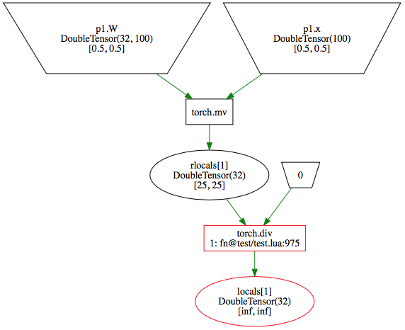
Consider this usage of autograd, it clearly contains a divide by zero.

local W = torch.Tensor(32,100):fill(.5)
local x = torch.Tensor(100):fill(.5)
local func = function(inputs)
   return torch.sum(torch.div(inputs.W * inputs.x, 0))  -- DIV ZERO!
end
local dFunc = autograd(func, {
   debugHook = function(debugger, msg)
      debugger.showDot()
      print(msg)
      os.exit(0)
   end
})
dFunc({W=W, x=x})

Will output:

autograd debugger detected a nan or inf value for locals[1]
   1: fn@path/to/code/example.lua:4

And render in Safari as:

Finer-grain control over execution can also be achieved using these flags:

-- All of these options default to true:
grad(f, {
   withForward = true | false,    -- compute the forward path
   withGradients = true | false,  -- compute the gradients (after forward)
   partialGrad = true | false     -- partial grad means that d(f) expects grads wrt output
})

-- Running this:
pred = grad(f, {withForward=true, withGradients=false})(inputs)
-- is equivalent to:
pred = f(inputs)
-- ... but the function is compiled, and benefits from tensor re-use!

License

Licensed under the Apache License, Version 2.0. See LICENSE file.