Technologicat/extrafeathers

Agility and ease-of-use batteries for the Python layer of the FEniCS finite element framework. The focus is on MPI-enabled 2D on P1, P2, P3, Q1, Q2, Q3, DP1, DP2, DP3, DQ1, DQ2, and DQ3 spaces. Each routine aims to be as general as is reasonable. Some of our utilities do support 3D meshes, but this is currently not a priority. Mesh import and closely related utilities run only serially.

Usage examples can be found in the demo/ subfolder.

The subpackage extrafeathers.pdes contains some modular ready-made solvers. These are mainly for use by the demos, but may be useful elsewhere. Particularly, stabilized Navier-Stokes and advection-diffusion solvers are provided.

Table of Contents

Features
Demos (with pictures!)
Questions & answers
- How to list the whole public API, and only the public API?
- What's up with the Unicode variable names?
Dependencies
Install & uninstall
- From source
License
Thanks

Features

Supported mesh dimensionalities are indicated in brackets. MPI is supported, unless indicated as "serial only".

Mesh-related utilities

cell_mf_to_expression [2D, 3D]
- Convert a scalar double MeshFunction into a CompiledExpression that can be used in UFL forms.
- For example, h = cell_mf_to_expression(meshsize(mesh)).
- For full examples, see extrafeathers.pdes.navier_stokes and extrafeathers.pdes.advection_diffusion, which use this in SUPG stabilization.
cellvolume [2D, 3D]
- Compute the local cell volume for the whole mesh.
- Convenience function; essentially just loops dolfin.Cell.volume over the mesh, and packs the result into a MeshFunction.
find_subdomain_boundaries [2D, 3D] [serial only]
- Automatically tag facets on internal boundaries between two subdomains. This makes it easier to respect DRY when setting up a small problem for testing, as the internal boundaries only need to be defined in one place (in the actual geometry).
- Tag also facets belonging to an outer boundary of the domain, via a callback function (that you provide) that gives the tag number for a given facet. This allows easily producing one MeshFunction with tags for all boundaries.
- Here subdomain means a SubMesh. These may result either from internal mesh generation via the mshr component of FEniCS, or from imported meshes. See the navier_stokes and import_gmsh demos for examples of both.
meshsize [2D, 3D]
- Compute the local mesh size (the h in finite element literature), defined as the maximum edge length of each mesh entity. The result is returned as a MeshFunction.
- Can compute both cell and facet meshfunctions.
- Useful for stabilization methods in advection-dominated problems, where h typically appears in the stabilization terms.
- See the import_gmsh demo for an example.
prepare_linear_export [2D]
- Exactly as it says on the tin, for P2, P3, Q2, Q3, DP2, DP3, DQ2, or DQ3 input data. Allows full nodal resolution export of degree-2 and degree-3 data into a vertex-based format (represented as refined degree-1 data).
- That is, given a P2, P3, Q2, Q3, DP2, DP3, DQ2, or DQ3 function space, prepare a degree-1 dolfin.Function on an appropriately refined mesh, and a DOF mapping that can be used to interpolate DOFs from the original space onto the DOFs of the degree-1 space.
- High-level function built on refine_for_export and map_coincident.
- See demo.coupled.main01_flow and demo.boussinesq.main01_solve for usage examples.
refine_for_export [2D], map_coincident [2D, 3D]
- These are the low-level functions that power prepare_linear_export.
- Prepare P2, P3, Q2, Q3, DP2, DP3, DQ2, or DQ3 (i.e. quadratic or cubic) data for export on a once-refined degree-1 mesh, so that it can be exported at full nodal resolution for visualization even when the file format is vertex-based.
  - Essentially, in a solver that does this, we want to w.assign(dolfin.interpolate(u, W)), where W (uppercase) is the once-refined degree-1 function space and w (lowercase) is a Function on it; this does work when running serially.
  - However, in parallel, the original and refined meshes will have different MPI partitioning (due to mesh editing to produce the refined mesh), so each process is missing access to some of the data it needs to compute its part of the interpolant. Hence we must construct a mapping between the global DOFs, allgather the whole original DOF vector, and then assign the data to the corresponding DOFs of w.
- refine_for_export differs from dolfin.refine in that for triangle meshes, we guarantee an aesthetically pleasing fill, which looks best for visualizing P2/P3 data, when interpolating that data as P1 on the refined mesh. Also, refine_for_export always produces a global refinement; every element is refined.
  - If you don't care about the aesthetics, for quadratic data, export_mesh = dolfin.refine(mesh) instead of export_mesh = extrafeathers.refine_for_export(mesh) works just as well.
- map_coincident is the low-level function that constructs a mapping between coincident DOFs on any two function spaces.
  - Supports both scalar and vector function spaces. Not tested on tensor fields yet.
  - Works with both continuous and discontinuous spaces. The practical difference is that for any scalar component of a continuous space, every DOF has a unique geometric location. In a discontinuous space, several distinct DOFs may share the same geometric location.
  - When both spaces (denoted V and W in the API) are discontinuous, the matching algorithm assumes that each cell on the mesh of W is contained in exactly one cell on the mesh of V; this allows a natural definition for "the same" DOF in the discontinuous case. The assumption is satisfied when the meshes are the same, or when W was produced by refining V. As a practically useful special case, when V uses quadrilateral elements, W may be the quad_to_tri of V.
  - The lower-level function _map_coincident does most of the work, and may be directly useful on special occasions. Differences to map_coincident:
    - Scalar function spaces only; .sub(j) of vector or tensor function space is accepted.
    - _map_coincident operates on the extrafeathers internal format: cells lists and nodes dictionaries, as produced by all_cells.
    - _map_coincident always returns the mappings in a multi-valued format, Dict[int, FrozenSet[int]]. Use extrafeathers.common.prune to auto-convert to single-valued Dict[int, int] in case all entries are actually single-valued.
    - _map_coincident performs no validation on its results.
- For full usage examples, see demo.coupled.main01_flow (vector), demo.coupled.main02_heat (scalar), and demo.boussinesq.main01_solve (both).
quad_to_tri [2D]
- Convert a quad mesh into a triangle mesh in crossed-diagonal format, by adding a node at each cell center and then replacing each quad by four triangles (that meet at the cell center node).
- This is used by mpiplot to make Matplotlib interpolate FEM functions on quadrilateral elements, by mapping the function onto an internal triangulation.
- Operates as a filter on the extrafeathers internal format. See the source code of plotmagic for full usage example.
patch_average, map_dG0
- map_dG0 [2D, 3D]:
  - Given a function space V and a dG0 function space W on the same mesh, determine the DOFs of W, and mesh cells, that form the support (mathematical sense) of each DOF of V.
  - Return two mappings:
    - Global V DOF number to an np.array of W DOF numbers.
    - Global W DOF number to cell index.
  - This is useful as a setup step for patch averaging.
- patch_average [2D, 3D]:
  - Given a scalar, vector or tensor function on a P1, P2 or P3 function space, patch-average it (weighted by relative cell volumes), and return the result as a new function on the same function space as the input.
  - This is sometimes useful as a postprocess step to eliminate some checkerboard modes, such as when using LBB-incompatible element types in a Navier-Stokes solver.
  - However, instead of patch-averaging, it is in general better to interpolate (or project) to a dG0 (elementwise constant) space and then just project back to the input (continuous) space:
```
import dolfin

W = dolfin.FunctionSpace(V.mesh(), "DG", 0)
f_averaged = dolfin.project(dolfin.interpolate(f, W), V)
```
    If V is a P1 space, the results are identical to patch-averaging; in all other cases, project(interpolate(...)) (or project(project(...))) does the same thing in spirit, but correctly.
    
    The patch_average function is provided just because patch-averaging is a classical postprocessing method.
specialize a meshfunction [2D, 3D] [serial only]
- Convert a MeshFunction on cells or facets of a full mesh into the corresponding MeshFunction on its SubMesh.
- Cell and facet meshfunctions supported.
- Useful e.g. when splitting a mesh with subdomains. This function allows converting the domain_parts and boundary_parts from the full mesh onto each submesh. This allows saving the submeshes, along with their subdomain and boundary tags, as individual standalone meshes in separate HDF5 mesh files. See the import_gmsh demo. This is useful, because (as of FEniCS 2019) SubMesh is not supported when running in parallel.
- See demo.import_gmsh for an example.
Low-level utilities; for more information, see docstrings:
- all_cells, all_patches, my_cells, my_patches [2D, 3D]
  - As of v0.4.0, the refine, vertices_only, and matplotlibize options of all_cells/my_cells are only available for 2D meshes.
- is_anticlockwise [2D]
  - Check whether a triplet of points in the plane is given in an anticlockwise order.
- make_mesh [2D, 3D]
  - Construct a dolfin.Mesh from arrays of cells and vertices, using dolfin.MeshEditor.
  - In MPI mode, can make a distributed mesh or an MPI-local mesh, as desired.
    - In some versions of FEniCS, some inputs may cause SCOTCH to crash when it attempts to MPI-partition the created mesh. Particularly, in FEniCS 2019, this is the case when the input data is the output of quad_to_tri. (That data works just fine in serial mode, and renumbering the nodes does not help.)
    - Constructing a quadrilateral mesh may fail with "cell is not orderable", even if there is just a single cell (even when extracted from a unit square quadrilateral mesh using all_cells and then fed back in to make_mesh). This is a known issue in DOLFIN [1] [2]; it should be fixed in DOLFINx, where the support for quadrilateral meshes has been improved significantly, but we do not support the next-gen FEniCS yet.
- trimesh [2D]
  - Triangulate the unit square using equilateral triangles (halves of them at two opposite edges).
- renumber_nodes_by_distance [2D]
  - As it says on the tin. May specify a custom origin; default is (min(x), min(y)).
  - Operates on the extrafeathers internal format.
- minmax [2D, 3D]
  - Extract the min and max of a FEM field on nodal elements. Modes available for raw, abs, l2 (euclidean length). When running in MPI mode, automatically gathers data from all processes. The data may live on an arbitrary subspace (e.g. a component of a vector field that itself lives on a MixedElement).

Plotting

mpiplot [2D]
- Plot the whole solution in the root process while running in parallel. For quick on-the-fly visualization.
  - The full mesh and function value data is automatically pieced together from all the MPI processes.
  - Degree-2 and degree-3 data is automatically converted onto a once-refined degree-1 mesh, to display it at full nodal resolution.
- P1, P2, P3, Q1, Q2, Q3, DP0, DP1, DP2, DP3, DQ0, DQ1, DQ2 and DQ3 elements supported.
- As of v0.4.0, scalar field only.
  - Note you can take a component of a vector or tensor field (.sub(j)), or interpolate an expression onto your function space, as usual. See demo.coupled.main01_flow for examples.
- Meant for debugging and visualizing simulation progress, especially for a lightweight MPI job that runs locally on a laptop (but still much faster with 4 cores rather than 1). Allows near-realtime visual feedback, and avoids the need to start ParaView midway through the computation just to quickly check if the solver is still computing and if the results look reasonable.
- Can optionally display the mesh and its MPI partitioning on top of the function data. See also mpiplot_mesh to do that separately.
mpiplot_mesh [2D]
- Plot the whole mesh in the root process while running in parallel.
- P1, P2, P3, Q1, Q2, Q3, DP0, DP1, DP2, DP3, DQ0, DQ1, DQ2 and DQ3 elements supported.
- Can optionally color-code the edges by MPI partitioning. Use matplotlib.pyplot.legend to see which is which.
- Can optionally display the visualization edges (generated by extrafeathers) of a degree-2 or degree-3 FunctionSpace, and the edges of the internal triangulation used for function interpolation on quadrilaterals. These are shown in a fainter color, to distinguish them from element edges.
plot_facet_meshfunction [2D] [serial only]
- Visualize whether the boundaries of a 2D mesh have been tagged as expected. Debug tool, for use when generating and importing meshes. This functionality is oddly missing from dolfin.plot.
- See demo.import_gmsh for an example.
Low-level utilities:
- as_mpl_triangulation [2D].
  - Represent the mesh of a scalar dolfin.FunctionSpace (or a component .sub(j) of a VectorFunctionSpace or TensorFunctionSpace) in Matplotlib format.
  - Has flags to refine degree-2 and degree-3 onto degree-1, and to represent the whole mesh or just the MPI-local part.
  - Produces both a matplotlib.tri.Triangulation (for function interpolation) as well as a matplotlib.collections.PolyCollection (element edges); and in the case of a quadrilateral mesh, some auxiliary data that can be used in mapping a function on the quads onto the triangulation (mpiplot uses this).
- pause
  - Non-focus-stealing pause helper for prodding Matplotlib into updating the figure window, courtesy of this StackOverflow post.

Mesh I/O

import_gmsh [2D, 3D] [serial only]
- Easily import a Gmsh mesh into FEniCS via meshio. Fire-and-forget convenience function for this common use case, to cover the gap created by the deprecation of the old dolfin-convert.
- Simplicial meshes (triangles, tetrahedra) only.
- Outputs a single HDF5 file with three datasets: /mesh, /domain_parts (physical cells i.e. subdomains), and /boundary_parts (physical facets i.e. boundaries).
read_hdf5_mesh [2D, 3D]
- Read in an imported mesh, and its physical cell and facet data.
- When running in parallel, we let FEniCS create a fresh MPI partitioning (so that it does not matter how many processes were running when the mesh file was written).
write_hdf5_mesh [2D, 3D]
- Write a mesh, and optionally its physical cell and facet data, in the same format as the output of import_gmsh.

Demos (with pictures!)

With a terminal in the top level directory of the project, demos are run as Python modules. This will use the version of extrafeathers in the source tree (instead of an installed one, if any).

Output of all demos will appear various subfolders of the demo/output/ folder, which is automatically created if not present.

Gmsh .msh files and the original .geo files to generate them can be found in the demo/meshes/ folder.

For judging the run time of the examples that display it on the screenshot, the demos were run in MPI mode, on four cores on a laptop with an Intel i7 4710-MQ @ 2.50 GHz CPU. Newer CPUs and especially desktop PCs are probably somewhat faster.

Peak memory usage was under 1GB for the four MPI processes in total, due to the 2D nature of the examples, and (for any but the most trivial examples) appropriately graded meshes to focus the allocation of DOFs into those parts of the domain where the resolution is actually needed.

DOF numbering related

Code: [global DOF numbering] [reference element]

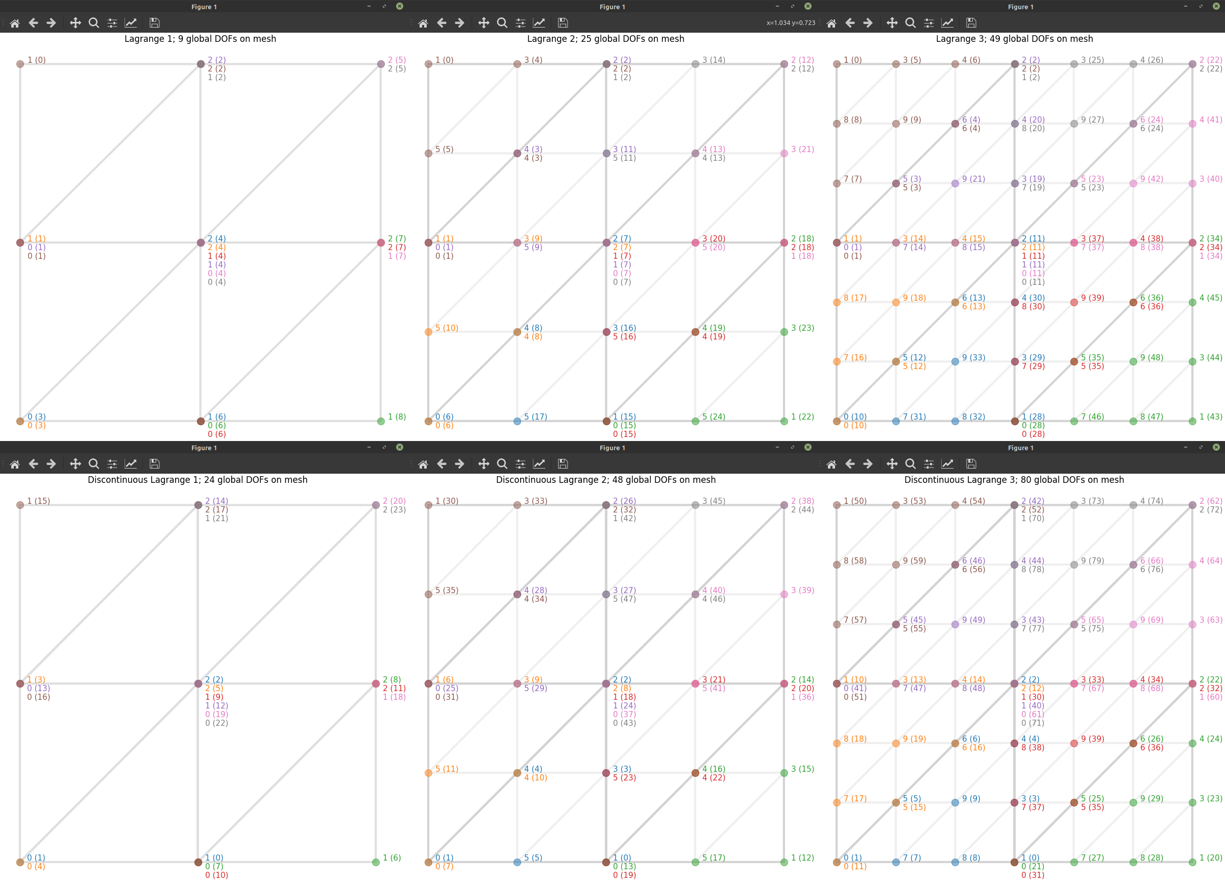
To illustrate how FEniCS numbers the global DOFs to maximize data locality (given that each process is allocated a contiguous chunk of DOFs):

python -m demo.dofnumbering
mpirun -n 2 python -m demo.dofnumbering
mpirun python -m demo.dofnumbering

Can also specify the element type:

python -m demo.dofnumbering P1
python -m demo.dofnumbering P2
python -m demo.dofnumbering P3
python -m demo.dofnumbering Q1
python -m demo.dofnumbering Q2
python -m demo.dofnumbering Q3
python -m demo.dofnumbering DP0
python -m demo.dofnumbering DP1
python -m demo.dofnumbering DP2
python -m demo.dofnumbering DP3
python -m demo.dofnumbering DQ0
python -m demo.dofnumbering DQ1
python -m demo.dofnumbering DQ2
python -m demo.dofnumbering DQ3

The strong lines are element edges; the faint lines indicate the automatically generated subdivisions for visualization of the P2 function as a once-refined P1 function. Each P2 triangle is split into four P1 triangles for visualization.

To see both the global and the reference-element DOF numbers on a 2×2 unit square mesh:

python -m demo.refelement

Can also specify the element type:

python -m demo.refelement P1
python -m demo.refelement P2
python -m demo.refelement P3
python -m demo.refelement Q1
python -m demo.refelement Q2
python -m demo.refelement Q3
python -m demo.refelement DP0
python -m demo.refelement DP1
python -m demo.refelement DP2
python -m demo.refelement DP3
python -m demo.refelement DQ0
python -m demo.refelement DQ1
python -m demo.refelement DQ2
python -m demo.refelement DQ3

Any of these works also in MPI mode, then color-coding the MPI partitioning by edge color. MPI-local node numbers (for the global DOFs) are not shown.

Reference-element and global DOF numbering for P1, P2, P3, DP1, DP2, and DP3 elements.

Patch averaging

[code]

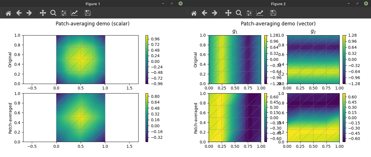
python -m demo.patch_average
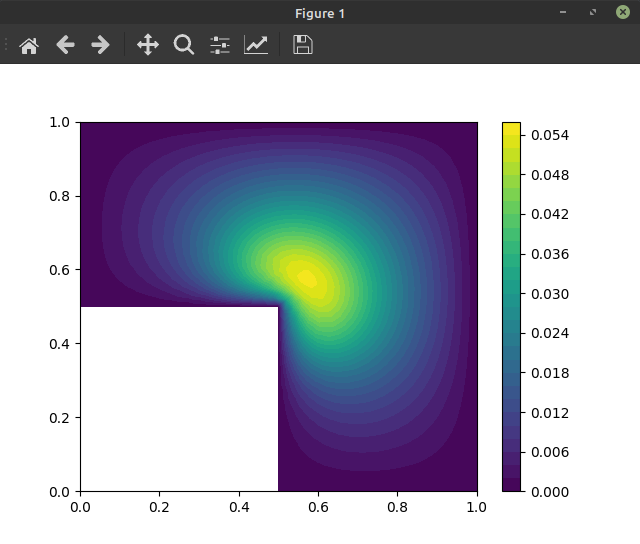
mpirun python -m demo.patch_average

Poisson equation

Code: [classic] [dG (SIPG)]

The classic: the Poisson equation with zero Dirichlet BCs, here on an L-shaped domain. Simple example of find_subdomain_boundaries and mpiplot.

python -m demo.poisson
mpirun python -m demo.poisson

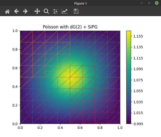
Poisson equation using symmetric interior penalty discontinuous Galerkin (SIPG) method. Example of cell_mf_to_expression and meshsize, as well as showing that mpiplot can plot the mesh (optionally, displaying its MPI partitioning) on top of the function data:

python -m demo.poisson_dg
mpirun python -m demo.poisson_dg

Poisson equation with dG(2) (a.k.a. DP2) elements. Note the visualization of the elements, and MPI mesh partitioning (4 processes: blue, orange, green, red, in that order).

Gmsh mesh import

[code]

python -m demo.import_gmsh

Physical groups are extracted by the importer. Here the fluid and structure meshes are imported into separate .h5 files.

Incompressible flow (Navier-Stokes)

Code: [mesh import] [solver]

With uniform mesh generated via mshr:

python -m demo.navier_stokes   # serial mode = generate HDF5 mesh file
mpirun python -m demo.navier_stokes   # parallel mode = solve

With a graded mesh imported from Gmsh (generated from demo/meshes/flow_over_cylinder.geo):

python -m demo.import_gmsh  # generate HDF5 mesh file, overwriting the earlier one
mpirun python -m demo.navier_stokes

The Gmsh mesh is recommended, to place the DOFs where they matter the most. Keep in mind Gresho & Sani (2000).

This Navier-Stokes demo supports solving only in parallel.

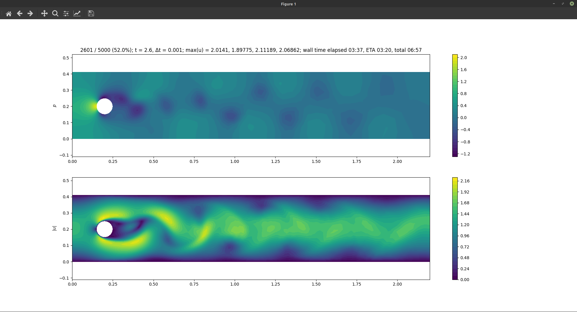
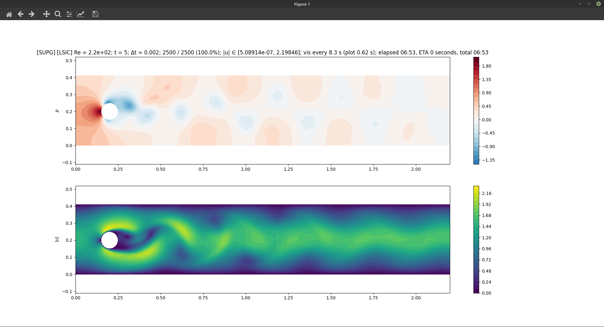
There is a more advanced version of the Navier-Stokes solver (with better modularization and factoring of the code, as well as three kinds of numerical stabilization) in extrafeathers.pdes.navier_stokes; for invoking it, see the forced convection demo below (demo.coupled.main01_flow).

Flow over a cylinder using P2P1 (Taylor-Hood) elements, i.e. P2 velocity and P1 pressure.

Forced convection (one-way coupled problem)

Code: [mesh import] [alt. mesh import] [internal mesh generation] [configuration] [flow solver] [heat solver]
Reusable PDEs: [Navier-Stokes] [heat equation]

This demo uses the same HDF5 mesh file as the Navier-Stokes demo, but comes with a more advanced Navier-Stokes solver with stabilization.

Create the mesh with one of:

python -m demo.import_gmsh  # graded mesh from Gmsh
python -m demo.coupled.main00_mesh  # internal uniform mshr mesh

If you want flow over two cylinders instead of just one, we provide another Gmsh mesh for that. To import it:

python -m demo.coupled.main00_alternative_mesh

The actual demo is run in two stages:

mpirun python -m demo.coupled.main01_flow
mpirun python -m demo.coupled.main02_heat

These solvers support both serial and parallel mode; parallel mode is recommended.

Be sure to wait until the flow simulation completes before running the heat simulation; the heat solver gets its advection velocity field from the timeseries file written by the flow solver.

Some simulation parameters can be found in demo.coupled.config, as well as the parameters for internal mshr mesh generation using demo.coupled.main00_mesh.

Convergence and accuracy:

With θ ≥ 1/2, the time integrator is A-stable. We use the skew-symmetric discretization for the advection term to allow this to work (Donea & Huerta, 2003, sec. 6.7.1).
As usual, stability does not imply accuracy; if the timestep is too large, the advection will skip over small-scale features in the flow field.
The solver can handle cases with pure Neumann boundary conditions on pressure (such as the standard cavity flow example). In these cases, we define the unique pressure field as that whose mean value is zero.
In the flow problem, a Dirichlet boundary condition on pressure (such as at an outlet) will force the pressure to reach its prescribed boundary value over one layer of elements.

Hence, it may be useful to deliberately use a low mesh resolution near the outlet, so that the discrete function space itself helps destroy any remaining nontrivial structure in the solution, before such structure gets an opportunity to hit the outflow boundary and cause a conflict with the boundary conditions (since that will often lead to a convergence failure). In an advection-dominated problem, the effects of this "smoothing by mesh geometry" on the upstream parts of the solution are negligible.
In the flow problem, LBB-compatible elements (e.g. P2P1) are recommended, but not mandatory. When P1 is used for velocity, the solver will postprocess the pressure field at the end of each timestep to eliminate checkerboard modes (which often arise as a symptom of LBB incompatibility).

However, note that for vector P1 elements, there are no divergence-free fields except the identically zero field (as pointed out by Brenner & Scott, 2010, p. 285), so when using P1 velocity, accuracy will suffer. During software testing of multiphysics solvers, P1 velocity may still be useful, as it runs much faster. (Can use P2 just for the final simulation.)

Flow over a cylinder using the improved, stabilized solver. P2P1 (Taylor-Hood) elements. SUPG and LSIC stabilization, and skew-symmetric advection.

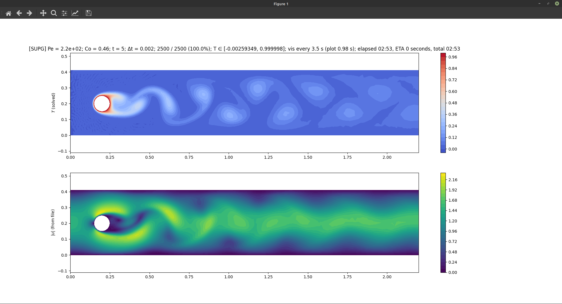
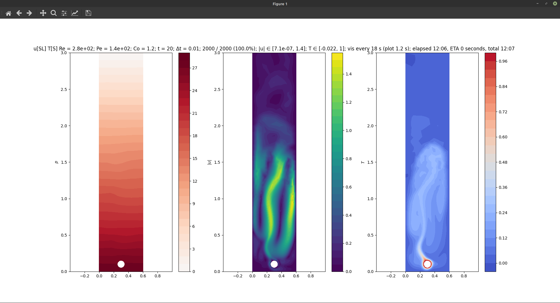
Forced convection over a hot cylinder kept at fixed temperature. Temperature field advected by the flow. P2 elements. SUPG stabilization and skew-symmetric advection.

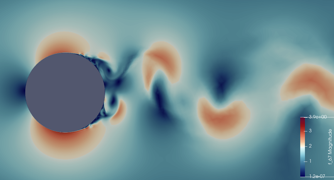
The advanced Navier-Stokes solver can survive at Re = 1.5e5, essentially producing a direct numerical simulation of turbulent flow. However, for accurate results, the mesh and timestep need to be much finer than those used here. This is using the "high Re setup" in the geometry file, and Δt = 2e-3. P2P1 elements, SUPG, LSIC, and skew-symmetric advection. Detail view of |u| near the cylinder. Visualized in ParaView.

Natural convection (two-way coupled problem)

Code: [mesh import] [configuration] [solver]
Reusable PDEs: [Navier-Stokes] [heat equation]

The model is based on the Boussinesq approximation. It uses the same Navier-Stokes solver as the forced convection demo, but now we add buoyancy via a Boussinesq source term for the velocity.

This demo has its own Gmsh mesh; see demo/meshes/cavity_with_obstacle.geo.

python -m demo.boussinesq.main00_mesh  # import Gmsh mesh
mpirun python -m demo.boussinesq.main01_solve

The solver supports both serial and parallel mode; parallel mode is recommended.

Some simulation parameters can be found in demo.boussinesq.config.

Natural convection induced by a hot cylinder kept at fixed temperature. We use a fine mesh for y ∈ [0, 0.75], and coarsen toward y = 3.0. Note the orientation; gravity has been added to the model, pointing down in the image. The Boussinesq approximation automatically generates the hydrostatic pressure. Flow solved using P2P1 (Taylor-Hood) elements, SUPG and LSIC stabilization, and skew-symmetric advection. Temperature solved using P2 elements, SUPG stabilization, and skew-symmetric advection.

Eulerian linear solid mechanics

Code: [mesh import] [internal mesh generation] [configuration] [solver]
Reusable PDE: [Eulerian linear solid]

Deformation of a sheet in two-dimensional space, with the sheet optionally subjected to axial motion.

The Eulerian view to solid mechanics - which is halfway between traditional solid mechanics and fluid mechanics, and commonly used in the analysis of process industry applications - is also known as axially moving materials. Our Eulerian displacement u is what Koivurova and Salonen (1999) term the mixed Lagrangean-Eulerian displacement. It is essentially an Eulerian quantity with the overall axial motion abstracted out; or in other words, u is the displacement from a reference state where the material moves uniformly at constant axial velocity.

For now, we provide the linear elastic and Kelvin-Voigt viscoelastic constitutive models. Future plans include the standard linear solid (SLS) and viscoplastic models (the latter of which requires major work; for reference, see the Julia package Materials.jl). However, when and whether this will happen depends on my work schedule. Right now the solver is provided as-is.

This "demo" is actually a small open-source research code into the mechanics of axially moving materials, with applications in the analysis of industrial processes. Placing the code here facilitates co-evolving extrafeathers with features our research team currently actually needs.

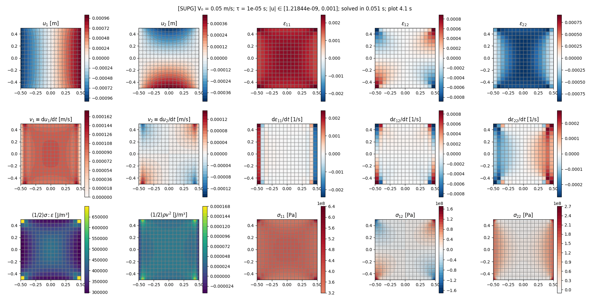
Steady state of axially moving 316L steel, in two dimensions, with a displacement-controlled pull of u₀ = 1e-3 m applied at the left and right edges. The top and bottom edges are free of tractions. From left to right, top to bottom, in that order: displacement u, infinitesimal strain tensor ε, material parcel velocity v = du/dt, Lagrangean strain rate dε/dt, volumetric elastic energy, volumetric kinetic energy, and the Cauchy stress tensor σ.

Constitutive law for linear viscoelastic materials in axial motion

For Eulerian descriptions of linear viscoelastic models, the axial motion introduces a third derivative in the strong form of the straightforward Eulerian description of the primal formulation (where we have a single PDE written in terms of u). Therefore, the weak form requires C1-continuous elements, which are not available in FEniCS, mainly for mathematical reasons outlined in Kirby & Mitchell (2019). The steady state of an axially moving Kelvin-Voigt sheet was solved in Kurki et al. (2016) using a custom C1 FEM code that was specialized to automatic discretization of PDEs on structured quadrilateral grids using Bogner-Fox-Schmit elements.

In this solver, we provide three different formulations that work with C0 elements:

In the straightforward Eulerian formulation, the unknowns are the displacement u, the Eulerian displacement rate v := ∂u/∂t, and the stress tensor σ.
In the alternative formulation, the unknowns are the displacement u, the material parcel velocity in the co-moving frame V := du/dt = ∂u/∂t + (a·∇)u, and the stress tensor σ.
In the primal formulation, the unknowns are the displacement u, and the material parcel velocity in the co-moving frame V := du/dt = ∂u/∂t + (a·∇)u. This is the recommended formulation.

In the straightforward formulation, the extra spatial derivative appears in the constitutive equation; in the other two, the definition of V absorbs it, and the equations resemble more the classical case without axial motion.

For illustration of the different approaches, consider the Kelvin-Voigt solid. With arbitrary elastic and viscous symmetry groups, the Kelvin-Voigt constitutive law reads

σ = E:ε + η:dε/dt

where E is the elastic stiffness tensor and η is the viscous stiffness tensor. Both tensors are rank-4, and satisfy the major and minor symmetries. As of v0.4.0, the material model implemented in the solver is isotropic, for which we can write the elastic stiffness tensor in Lamé format as

E = 2μS + 3λV

The tensors S and V are the symmetric and volumetric rank-4 identity tensors; μ is the shear modulus, and λ is the first Lamé parameter. For any rank-2 tensor T, the tensors S and V satisfy the projection relations

S:T = symm(T)
V:T = vol(T) ≡ (1/3) I tr(T)

These are indeed projections; the operators S:(...) and V:(...) are idempotent.

To simplify the model (thus also reducing requirements on experimental data we must acquire to be able to use the model), we assume that the elastic and viscous stiffnesses behave similarly, differing only by a scaling factor. We define the viscous stiffness tensor η in terms of E and the Kelvin-Voigt retardation time τ as

η = τ E

Physically, τ is related to the creep rate. Note in one space dimension, one commonly writes τ := η / E, but the above alternative definition works also in 2D and 3D.

Since the constitutive law holds at a material point, in the Eulerian representation we have d/dt = ∂/∂t + a·∇, where a is the drive velocity field (assumed constant in space) that describes the axial motion. Now there are at least two possibilities to handle this.

Formulation used in `EulerianSolid`

A straightforward Eulerian representation of the constitutive law is

σ = E:ε + η:(∂ε/∂t + a·∇ε)

where ε is the Eulerian description of the strain. To obtain the strain, in the small-displacement regime, the kinematic relation is

εij = (symm ∇u)ij ≡ (1/2) (∂i uj + ∂j ui)

Using an Eulerian description for the displacement u, we get the Eulerian ε.

Because we represent u by C0-continuous elements, ∇u is discontinuous across element boundaries. Therefore, ε is discontinuous across element boundaries, and in order for the weak form to remain integrable (without introducing jump terms), we are not allowed to take spatial derivatives of ε.

To overcome this, we integrate by parts in the a·∇ε term, moving the directional derivative a·∇ onto the test function. The weak form of the constitutive law reads

∫ φ:σ dx = ∫ φ:E:ε dx + ∫ φ:η:(∂ε/∂t + a·∇ε) dx

where φ is a rank-2 test tensor (virtual strain), and ∫ ... dx denotes integration over the domain. The appropriate integration-by-parts formula is

∫ φ:η:[(a·∇)ε] dx = ∫ (a·n) (φ:η:ε) dΓ - ∫ [(a·∇)φ]:η:ε dx - ∫ φ:[(a·∇)η]:ε dx - ∫ (∇·a) (φ:η:ε) dx

where ∫ ... dΓ denotes integration over the boundary of the domain, φ and ε are rank-2 tensors, η is a rank-4 tensor that satisfies the major symmetry, and a is a vector. (The formula is easily shown using the divergence theorem.)

The axial drive velocity field is divergence-free, so the last term vanishes. If η is constant in space, also the second-to-last term vanishes, and we have

∫ φ:η:[(a·∇)ε] dx = ∫ (a·n) (φ:η:ε) dΓ - ∫ [(a·∇)φ]:η:ε dx

The weak form of the constitutive law becomes

∫ φ:σ dx = ∫ φ:E:ε dx + ∫ φ:η:∂ε/∂t dx - ∫ [(a·∇)φ]:η:ε dx + ∫ (a·n) (φ:η:ε) dΓ

Using the definition η = τ E, we obtain

∫ φ:σ dx = ∫ φ:E:ε dx + τ ∫ φ:E:∂ε/∂t dx - τ ∫ [(a·∇)φ]:E:ε dx + τ ∫ (a·n) (φ:E:ε) dΓ

Note we have applied integration by parts on the right-hand side of the constitutive equation. Therefore, the boundary term does not represent a boundary condition for σ; it should be evaluated as-is.

With this integration by parts, there is no need to spatially differentiate ε. All terms are integrable across element boundaries even when u is represented by C0-continuous elements. The SLS model can be treated similarly.

In practice, though, it was observed that it is better for numerical stability to project symm ∇u and symm ∇v into a C0-continuous space before using the data in the constitutive equation. Since the projected fields are once differentiable, this allows us to actually integrate by parts in only "half" of the (a·∇)ε term, enabling the use of the numerically more stable skew-symmetric representation for the weak form of the advection operator. See the functions advw and advs in module extrafeathers.pdes.numutil.

The stress tensor is then used in the straightforward Eulerian representation of the momentum balance:

ρ ∂²u/∂t² + 2 ρ (a·∇) ∂u/∂t + ρ (a·∇)(a·∇)u - ∇·σ = ρ b

which is written in the laboratory frame.

Formulation used in `EulerianSolidAlternative`

The alternative formulation takes as its velocity-like variable the material parcel velocity, as measured against the co-moving frame. This simplifies the equations somewhat. Let

V := du/dt
   = ∂u/∂t + (a·∇) u

Note we are skipping some important details here; u is an Eulerian field in the laboratory frame, whereas V - although we write it in a laboratory-frame Eulerian description - is the actual physical velocity of the material parcels with respect to the co-moving frame.

Conveniently, V is also the Lagrangean displacement rate with respect to the state with uniform axial motion. Since the uniform axial motion causes no strains, we can use V to derive the Lagrangean strain rate dε/dt. The constitutive law becomes

σ = E : ε + η : dε/dt
  = E : (symm ∇u) + η : d/dt (symm ∇u)
  = E : (symm ∇) u + η : d/dt (symm ∇) u
  = E : (symm ∇) u + η : (symm ∇) du/dt
  = E : (symm ∇) u + η : (symm ∇) V
  = E : (symm ∇) u + τ E : (symm ∇) V
  =: ℒ(u) + τ ℒ(V)

which is of the same form as the standard Lagrangean constitutive law, but this law is actually Eulerian. Both u and V are written using Eulerian descriptions in the laboratory frame, and also the ∇ is taken in spatial coordinates. There is no axial motion term, because it is absorbed by the definition of V.

Since we are modeling a viscoelastic solid, we need the displacement u. It is obtained by solving the first-order transport PDE

∂u/∂t + (a·∇) u = V

or in other words, we use the laboratory-frame Eulerian description of V to update the laboratory-frame Eulerian description of u.

In this formulation, the Eulerian linear momentum balance in the laboratory frame is just

ρ ∂V/∂t + ρ (a·∇) V - ∇·σ = ρ b

which resembles Navier-Stokes, but now σ is the stress tensor for a solid. The advection operator has a different velocity field here, because in this model, the material parcel velocity with respect to the laboratory frame is v := a + V. Here a is a constant field, and V is a first-order small quantity. Hence in the laboratory frame, we obtain the form above.

Formulation used in `EulerianSolidPrimal`

Like EulerianSolidAlternative, but with the primal variables u and V only. Like in our implementation of Navier-Stokes, the stress tensor is treated by inserting its expression into the linear momentum balance.

Again, V is the Eulerian field that represents the actual physical material parcel velocity in the co-moving frame.

The equations are, as in EulerianSolidAlternative,

V = du/dt
  = ∂u/∂t + (a·∇) u

σ = E : ε + η : dε/dt
  = ℒ(u) + τ ℒ(V)

ρ ∂V/∂t + ρ (a·∇) V - ∇·σ = ρ b

but now instead of introducing another function space for σ, we just insert its expression in terms of u and V into the linear momentum balance.

This allows us to use a Neumann boundary condition for the stress, which is much better for setting the traction vector n·σ on boundaries of arbitarily shaped domains.

Also, we switch the roles of the first and third equations; we use the linear momentum balance to determine u, and use the first equation to define V simply as the L² projection of du/dt, so in this formulation, V itself needs no boundary conditions.

Notes on the numerical scheme

The main points are given below. Many more technical details are documented in the docstrings and in source code comments.

In all three dynamic solvers, time integration is performed with the θ method, defaulting to Crank-Nicolson (θ = 1/2).

As of v0.4.0:

SteadyStateEulerianSolidPrimal is the only working steady-state solver.
All three dynamic solvers work fine, although EulerianSolidPrimal is the cleanest formulation and the fastest solver, and thus recommended.
There are still some issues in getting cases with pure traction boundary conditions to work properly.
- As a workaround, use boundary conditions inside the domain to fix the displacement at some appropriate location (and make sure that in the mesh, there actually are DOFs sufficiently near the coordinates where you are fixing the displacement). There is an example of how to do this in demo.euleriansolid.main01_solve.

`EulerianSolid` and `EulerianSolidAlternative`

Each timestep of the dynamic simulation is solved iteratively:

Update u using the latest available v.
Solve σ from the constitutive law.
Solve v from the linear momentum balance equation, using σ and u.
If ||v - v_prev||_H1 < tol, the timestep is complete; else jump back to item 1.

In EulerianSolid, u does not take boundary conditions, because u is just the time integral of v. Instead, one should set an initial field for u, and then set the boundary conditions for v appropriately. If you want a prescribed displacement at a boundary, that should be fed in as the initial condition for u.

In EulerianSolidAlternative, when V0 ≠ 0, u needs boundary conditions on the inflow part of the boundary (defined as those segments of ∂Ω on which a·n < 0, where a := (V0, 0)). Of course it is additionally possible to provide an initial field for u.

The function space for the stress must be sufficiently large compared to that for the displacement. With Q1 displacement, Q2 stress works fine. (Respectively P1/P2 on triangles.)

In these algorithms, there is a stability limit for the timestep size. It has not yet been investigated whether this arises due to the iterative splitting, or due to the introduction of the extra function space for the stress.

`EulerianSolidPrimal`

Each timestep of the dynamic simulation is solved as a monolithic equation system, where both u and V are treated as unknowns simultaneously. Both fields use a copy of the same function space; Q1 works fine. (Respectively P1 on triangles.)

Boundary conditions should be set on u. In this formulation, V takes no boundary conditions.

Any boundary that has no condition on u will use a Neumann boundary condition for the traction vector n·σ₀, where σ₀ is a prescribed boundary stress. The boundary stress field must be supplied when instantiating the solver. There is only one, but it can be any object that can be used in an UFL form (so for complex cases, a FEM field on the same mesh is fine).

Note in this solver you can also set just one component of u, if you want; the other component will then use the Neumann boundary condition on stress.

The dynamic solver uses MUMPS (Multifrontal Massively Parallel Sparse direct solver) to solve the linear equation system, as it seems this system is not amenable to any combination of Krylov solver and preconditioner available in FEniCS. (Note that for a ≠ 0, the system is not symmetric due to the (a·∇) terms, so only non-symmetric methods are applicable.)

Just like the other algorithms, the solver computes the strain and stress fields, but this is done as a postprocessing step. These fields are provided for visualization only; they are not used during the solution process.

Having the equations as one monolithic system allows A-stability in time integration. Keep in mind that as always, a reasonably small timestep size is nevertheless recommended to obtain reasonable simulation quality. If you want to converge quickly to the steady state, use the steady-state solver SteadyStateEulerianSolidPrimal instead.

Running the demo

The recommended way to run the demo is

python -m demo.euleriansolid.main00_alternative_mesh  # generate quad mesh
mpirun python -m demo.euleriansolid.main01_solve

Then load up the results in ParaView. Displacement, stress tensor, and the von Mises stress are exported.

In addition, all plotted figures from during the simulation are auto-saved as images.

The solver can also run using an unstructured triangle mesh (generated from demo/meshes/box.geo):

python -m demo.euleriansolid.main00_mesh  # import Gmsh mesh
mpirun python -m demo.euleriansolid.main01_solve

However, as one may generally expect, the regular quad mesh does give better accuracy when the domain is the unit square.

References:

Robert C. Kirby and Lawrence Mitchell. 2019. Code generation for generally mapped finite elements. ACM Transactions on Mathematical Software 45(41), 1-23. https://doi.org/10.1145/3361745 https://arxiv.org/abs/1808.05513

H. Koivurova and E.-M. Salonen. 1999. Comments on non-linear formulations for travelling string and beam problems. Journal of Sound and Vibration 255(5), 845-856.

Matti Kurki, Juha Jeronen, Tytti Saksa, and Tero Tuovinen. 2016. The origin of in-plane stresses in axially moving orthotropic continua. International Journal of Solids and Structures 81, 43-62. https://doi.org/10.1016/j.ijsolstr.2015.10.027

Questions & answers

How to list the whole public API, and only the public API?

In short, use Python's introspection capabilities. There are some subtleties here; below are some recipes.

To view the public API of a given submodule:

import sys
print(sys.modules["extrafeathers.meshmagic"].__all__)  # for example

If the __all__ attribute for some submodule is missing, that submodule has no public API.

To view the whole public API, grouped by submodule:

import sys

import extrafeathers

submodules = [name for name in dir(extrafeathers)
              if f"extrafeathers.{name}" in sys.modules]

for name in submodules:
    module = sys.modules[f"extrafeathers.{name}"]
    if hasattr(module, "__all__"):  # has a public API?
        print("=" * 79)
        print(f"Public API of extrafeathers.{name}':")
        print(module.__all__)

Do not do this to retrieve the submodules:

import types
submodules_wrong = [name for name in dir(extrafeathers)
                    if issubclass(type(getattr(extrafeathers, name)), types.ModuleType)]

because generally speaking, it is subtly wrong. If there happens to be an object imported from a submodule that has the same name as the submodule itself, that submodule will be missing from the list, because the object overrides the submodule in the parent module's namespace. The first approach is correct and always works.

To view the whole public API available in the top-level namespace:

import types

import extrafeathers

non_module_names = [name for name in dir(extrafeathers)
                    if not issubclass(type(getattr(extrafeathers, name)), types.ModuleType)]
print(non_module_names)

Now be very very careful: for the same reason as above, for the correct semantics we must use issubclass(..., types.ModuleType), not ... in sys.modules. Here we want to list each symbol in the top-level namespace of extrafeathers that does not point to a module; including any objects that override a module in the top-level namespace.

What's up with the Unicode variable names?

Looks more like math to use ρ instead of rho. Too bad Python doesn't accept ∇ or ∂ in variable names; with those, the PDEs would look even better.

To type Unicode greek symbols, use an IME such as latex-input, or Emacs's counsel-unicode-char (from the counsel package; on its features, see this blog post).

Dependencies

Beside the Python-based requirements in requirements.txt, this depends on libhdf5 (backend for h5py) and fenics, which are not Python packages. You'll likely also want OpenMPI to run FEniCS on multiple cores (though fenics likely already pulls that in).

On Ubuntu-based systems,

sudo apt install libhdf5-dev libopenmpi-dev fenics

should install them. extrafeathers was developed using libhdf5-103, openmpi 4.0.3, and fenics 2019.2.0.5.

If h5py fails to install, or crashes when trying to read/write HDF5 files, try recompiling it against the libhdf5 headers you have; see the build instructions.

If you want to modify the .geo files and generate new meshes for some of the demos, you'll need Gmsh.

Additionally, ParaView is useful for visualizing the XDMF output files from FEniCS.

Install & uninstall

From source

Clone the repo from GitHub. Then, navigate to it in a terminal, and:

python -m setup install

possibly with --user, if your OS is a *nix, and you feel lucky enough to use the system Python. If not, activate your venv first; the --user flag is then not needed.

To uninstall:

pip uninstall extrafeathers

but first, make sure you're not in a folder that has an extrafeathers subfolder - pip will think it got a folder name instead of a package name, and become confused.

License

Starting at v0.2.0, all original code in this repository is licensed under the 2-clause BSD license.

A very large majority of the code is original. Any code fragments from forums are licensed by their respective authors under the terms the particular forum places on code contributions. In the case of StackOverflow, this means the fragments are used under the CC-BY-SA license. Attribution is given by providing the forum post URL and username in the source code comments.

Thanks

Everyone who has posted solutions on the old FEniCS Q&A forum (now archived) and the discourse group; especially @Dokken. These resources were great for getting started.

Technologicat / extrafeathers

Features

Mesh-related utilities

Plotting

Mesh I/O

Demos (with pictures!)

DOF numbering related

Patch averaging

Poisson equation

Gmsh mesh import

Incompressible flow (Navier-Stokes)

Forced convection (one-way coupled problem)

Natural convection (two-way coupled problem)

Eulerian linear solid mechanics

Constitutive law for linear viscoelastic materials in axial motion

Formulation used in `EulerianSolid`

Formulation used in `EulerianSolidAlternative`

Formulation used in `EulerianSolidPrimal`

Notes on the numerical scheme

`EulerianSolid` and `EulerianSolidAlternative`

`EulerianSolidPrimal`

Running the demo

Questions & answers

How to list the whole public API, and only the public API?

What's up with the Unicode variable names?

Dependencies

Install & uninstall

From source

License

Thanks

About

Languages

Features

Mesh-related utilities

Plotting

Mesh I/O

Demos (with pictures!)

DOF numbering related

Patch averaging

Poisson equation

Gmsh mesh import

Incompressible flow (Navier-Stokes)

Forced convection (one-way coupled problem)

Natural convection (two-way coupled problem)

Eulerian linear solid mechanics

Constitutive law for linear viscoelastic materials in axial motion

Formulation used in EulerianSolid

Formulation used in EulerianSolidAlternative

Formulation used in EulerianSolidPrimal

Notes on the numerical scheme

EulerianSolid and EulerianSolidAlternative

EulerianSolidPrimal

Running the demo

Questions & answers

How to list the whole public API, and only the public API?

What's up with the Unicode variable names?

Dependencies

Install & uninstall

From source

License

Thanks

About

Languages

Formulation used in `EulerianSolid`

Formulation used in `EulerianSolidAlternative`

Formulation used in `EulerianSolidPrimal`

`EulerianSolid` and `EulerianSolidAlternative`

`EulerianSolidPrimal`