Finite Element Model - Matlab Toolbox

Introduction

This small toolbox provides a set of functions to help using flexible elements on Simscape from a Finite Element Software.

The functions are all described in section sec:functions.

Few examples are provided in the following sections.

Import Flexible Elements in Simscape using Component Mode Synthesis in Ansys

Introduction

In this section, we wish to model a simple flexible cantilever beam using Simscape.

The cantilever beam is first defined in Ansys. The reduced Mass and Stiffness matrices are then exported using the Component Mode Synthesis.

The coordinates of interface nodes (nodes where forces can be applied, displacements measured, and connections with other elements) are also exported.

First, these information are imported in Matlab, and then are used in Simscape to model the flexible element.

Matlab Init

addpath('./src/');
addpath('examples/cant_beam/');

Import Mass Matrix, Stiffness Matrix, and Interface Nodes Coordinates

We first extract the stiffness matrix.

K = extractMatrix('cant_beam_K.txt');

42000.0	0.0	0.0	0.0	0.0	0.0	-42000.0	0.0	0.0	0.0
0.0	17.0	0.0	0.0	0.0	4200.0	0.0	-17.0	0.0	0.0
0.0	0.0	17.0	0.0	-4200.0	0.0	0.0	0.0	-17.0	0.0
0.0	0.0	0.0	230000.0	0.0	0.0	0.0	0.0	0.0	-230000.0
0.0	0.0	-4200.0	0.0	1400000.0	0.0	0.0	0.0	4200.0	0.0
0.0	4200.0	0.0	0.0	0.0	1400000.0	0.0	-4200.0	0.0	0.0
-42000.0	0.0	0.0	0.0	0.0	0.0	84000.0	0.0	0.0	0.0
0.0	-17.0	0.0	0.0	0.0	-4200.0	0.0	34.0	0.0	0.0
0.0	0.0	-17.0	0.0	4200.0	0.0	0.0	0.0	34.0	0.0
0.0	0.0	0.0	-230000.0	0.0	0.0	0.0	0.0	0.0	460000.0

M = extractMatrix('cant_beam_M.txt');

0.00013	0.0	0.0	0.0	0.0	0.0	6.5e-05	0.0	0.0	0.0
0.0	0.00014	0.0	0.0	0.0	0.01	0.0	5e-05	0.0	0.0
0.0	0.0	0.00014	0.0	-0.01	0.0	0.0	0.0	5e-05	0.0
0.0	0.0	0.0	0.0022	0.0	0.0	0.0	0.0	0.0	0.0011
0.0	0.0	-0.01	0.0	0.93	0.0	0.0	0.0	-0.006	0.0
0.0	0.01	0.0	0.0	0.0	0.93	0.0	0.006	0.0	0.0
6.5e-05	0.0	0.0	0.0	0.0	0.0	0.00026	0.0	0.0	0.0
0.0	5e-05	0.0	0.0	0.0	0.006	0.0	0.00029	0.0	0.0
0.0	0.0	5e-05	0.0	-0.006	0.0	0.0	0.0	0.00029	0.0
0.0	0.0	0.0	0.0011	0.0	0.0	0.0	0.0	0.0	0.0043

Then, we extract the coordinates of the interface nodes.

[int_xyz, int_i] = extractNodes('cant_beam.txt');

Node Number	x	y	z
1	0	0	0
6	500	0	0
22	1000	0	0

Using K, M and int_xyz, we can use the Reduced Order Flexible Solid simscape block.

Identification of the Dynamics

The flexible element is imported using the Reduced Order Flexible Solid simscape block.

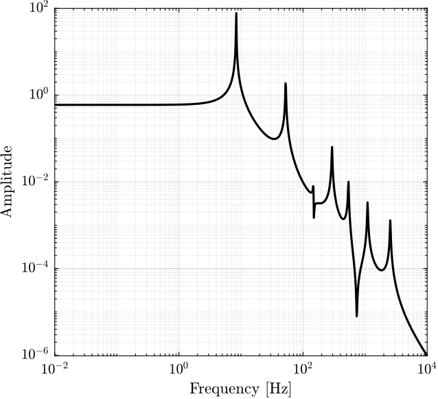
The beginning of the cantilever beam is fixed to the World frame, a force actuator is added in the z direction on the middle node, and a z-displacement sensor is added at the end of the beam.

The dynamics is identified from the applied force to the measured displacement (Figure fig:cant_beam_frf).

%% Name of the Simulink File
mdl = 'cant_beam';

%% Input/Output definition
clear io; io_i = 1;
io(io_i) = linio([mdl, '/F'], 1, 'openinput');  io_i = io_i + 1;
io(io_i) = linio([mdl, '/z'], 1, 'openoutput'); io_i = io_i + 1;

G = linearize(mdl, io);

Low Order Dynamical Model from a Finite Element Model

Introduction

Most of the example presented in this section are taken from cite:hatch00_vibrat_matlab_ansys.

The goal is to obtain a low order model from a Finite Element Model.

We suppose here that the eigenvalues and eigenvectors are exported using a Finite Element software.

Once the eigenvalues and eigenvectors are imported, one should choose the inputs and outputs nodes (e.g. where the forces and the displacements are measured) to first reduce the number of eigenvectors.

Damping can then be added to each.

Then, in order to reduce the size of the model, only few modes are included in the model. The selection of the modes to keep in the model can be based on the “dc gain” or “peak gain” method depending on the damping.

Finally, the full model and reduced models are compared.

Matlab Init

addpath('./src/');
addpath('examples/cant_beam_ansys/');

Extract Eigenvalues and Eigenvectors

The eigenvalues and eigenvectors are extracted.

[xn, f0] = extractEigs('cantbeam30bl.eig', 'dirs', [1 0 0 0 0 0]');

n_nodes = size(xn, 1);
n_modes = size(xn, 2);

Define Physical Inputs and Outputs

First, define the node numbers corresponding to the inputs and outputs

i_input = 14; % middle of the beam
i_output = 29; % end of the beam

Define Damping

We here use uniform damping.

xi = 0.01;

All Modes Included in the Model

The state space matrices are created by “inspection”. Here, we include all the modes.

System Matrix - A

Adiag = zeros(2*n_modes,1);
Adiag(2:2:end) = -2*xi.*(2*pi*f0);

Adiagsup = zeros(2*n_modes-1,1);
Adiagsup(1:2:end) = 1;

Adiaginf = zeros(2*n_modes-1,1);
Adiaginf(1:2:end) = -(2*pi*f0).^2;

A = diag(Adiag) + diag(Adiagsup, 1) + diag(Adiaginf, -1);

System Matrix - B

B = zeros(2*n_modes, length(i_input));

for i = 1:length(i_input)
    % Physical Coordinates
    Fp = zeros(n_nodes, 1);
    Fp(i_input(i)) = 1;

    B(2:2:end, i) = xn'*Fp;
end

System Matrix - C

C = zeros(length(i_output), 2*n_modes);
C(:, 1:2:end) = xn(i_output, :);

System Matrix - D

D = zeros(length(i_output), length(i_input));

State Space Model

G_f = ss(A, B, C, D);

Simple mode truncation

Let see what happens is we simply truncate the number of modes (keeping only the low frequency modes).

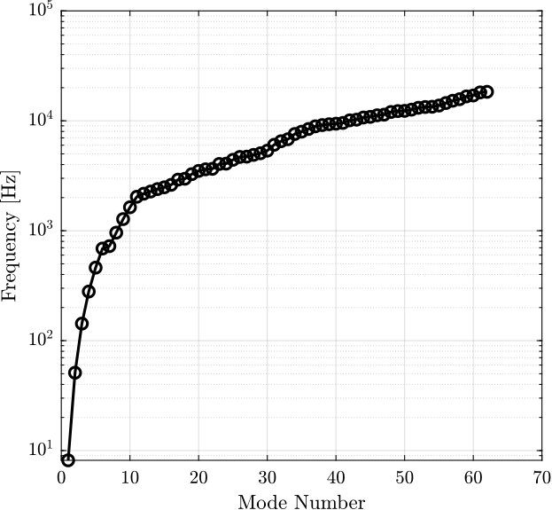
The frequency of the modes are shown in Figure fig:hatch00_cant_beam_modes_freq.

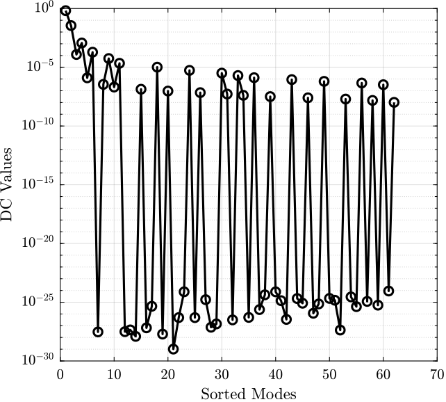
The DC gain of each mode is shown in Figure fig:hatch00_cant_beam_unsorted_dc_gains.

Let’s keep only the first 10 modes.

m_max = 10;
xn_t = xn(:, 1:m_max);
f0_t = f0(1:m_max);

And create the state space model with the kept modes:

Modes sorted by their DC gain

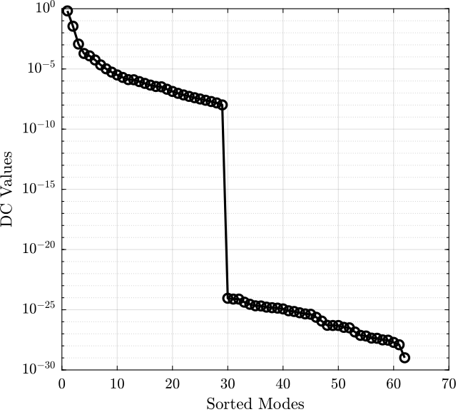
Let’s sort the modes by their DC gains and plot their sorted DC gains (Figure fig:hatch00_cant_beam_sorted_dc_gains).

dc_gain = abs(xn(i_input, :).*xn(i_output, :))./(2*pi*f0).^2;

[dc_gain_sort, index_sort] = sort(dc_gain, 'descend');

Let’s keep only the first 10 sorted modes.

m_max = 10;

xn_s = xn(:, index_sort(1:m_max));
f0_s = f0(index_sort(1:m_max));

And create the state space model with the kept modes:

G_s = ss(A, B, C, D);

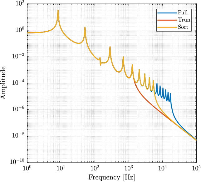
Comparison

The following models are compared on Figure fig:cant_beam_comp_reduc_techniques:

full model containing all the modes
the truncated model containing only the low frequency modes
the model where modes are sorted based on DC gain before selection

One can see that with the same number of modes, the sorted model gives much better results than the truncated one.

Effect of the Individual Modes

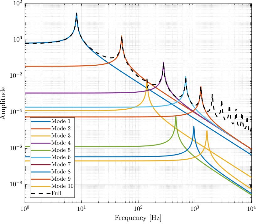
To see why it is better to sort the modes prior mode reduction, we can look at the contribution of the individual modes as shown in Figure fig:cant_beam_individial_modes.

One can see that some modes have no effect on the dynamics for the selected inputs and outputs.

freqs = logspace(0, 4, 1000);

figure;
hold on;
for mode_i = 1:10
    A = zeros(2);
    A(2,2) = -2*xi.*(2*pi*f0(mode_i));
    A(1,2) = 1;
    A(2,1) = -(2*pi*f0(mode_i)).^2;

    B = [0; xn(i_input, mode_i)'];

    C = [xn(i_output, mode_i), 0];

    D = zeros(length(i_output), length(i_input));

    plot(freqs, abs(squeeze(freqresp(ss(A,B,C,D), freqs, 'Hz'))), ...
         'DisplayName', sprintf('Mode %i', mode_i));
end
plot(freqs, abs(squeeze(freqresp(G_f, freqs, 'Hz'))), 'k--', ...
     'DisplayName', 'Full');
set(gca, 'XScale', 'log'); set(gca, 'YScale', 'log');
ylabel('Amplitude'); xlabel('Frequency [Hz]');
ylim([1e-9, 1e2]);
legend('location', 'southwest');

Non-Uniform Damping

Definition of the Damping

Let’s say we want to use Rayleigh damping: \begin{equation} ξ_i = \frac{a + b ω_i^2}{ω_i} \end{equation}

We define the parameters on Matlab:

a = 1e-2;
b = 1e-6;
xi = (a + b * (2*pi*f0).^2)./(2*pi*f0);

State Space Model

And we can create the state space model.

System Matrix - A

Adiag = zeros(2*n_modes,1);
Adiag(2:2:end) = -2*xi.*(2*pi*f0);

Adiagsup = zeros(2*n_modes-1,1);
Adiagsup(1:2:end) = 1;

Adiaginf = zeros(2*n_modes-1,1);
Adiaginf(1:2:end) = -(2*pi*f0).^2;

A = diag(Adiag) + diag(Adiagsup, 1) + diag(Adiaginf, -1);

System Matrix - B

B = zeros(2*n_modes, length(i_input));

for i = 1:length(i_input)
    % Physical Coordinates
    Fp = zeros(n_nodes, 1);
    Fp(i_input(i)) = 1;

    B(2:2:end, i) = xn'*Fp;
end

System Matrix - C

C = zeros(length(i_output), 2*n_modes);
C(:, 1:2:end) = xn(i_output, :);

System Matrix - D

D = zeros(length(i_output), length(i_input));

State Space Model

G_d = ss(A, B, C, D);

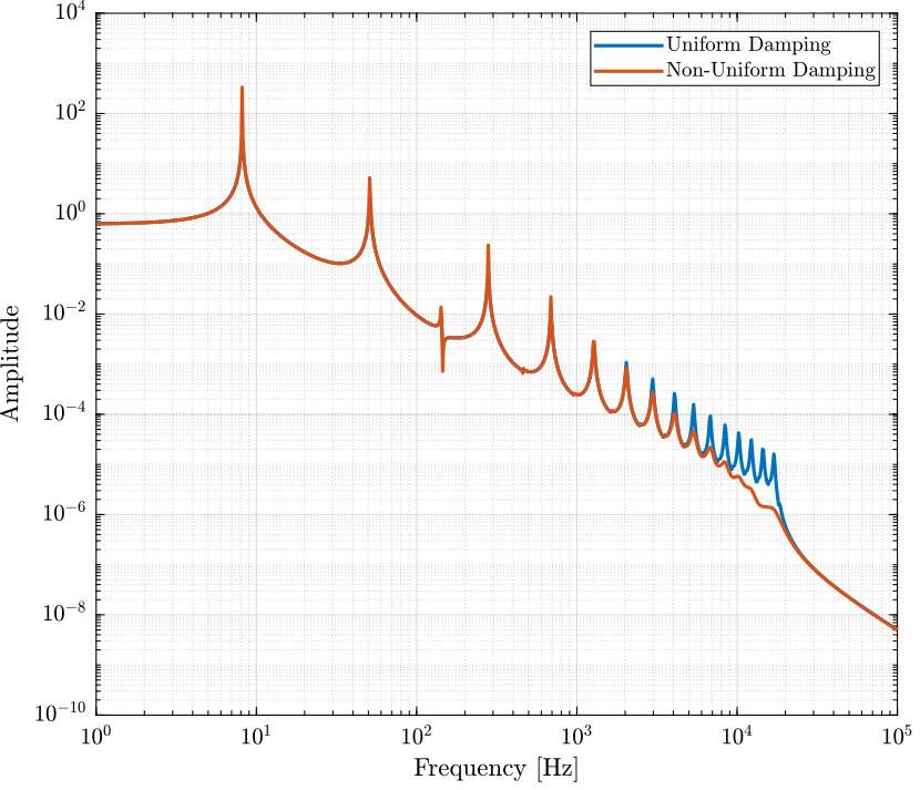
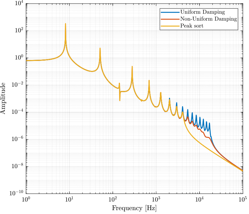
Obtained Dynamics

And we compare the obtained dynamics when using Uniform Damping (Figure fig:cant_beam_comp_unif_non_unif_damp).

Sort Modes based on their peak gain

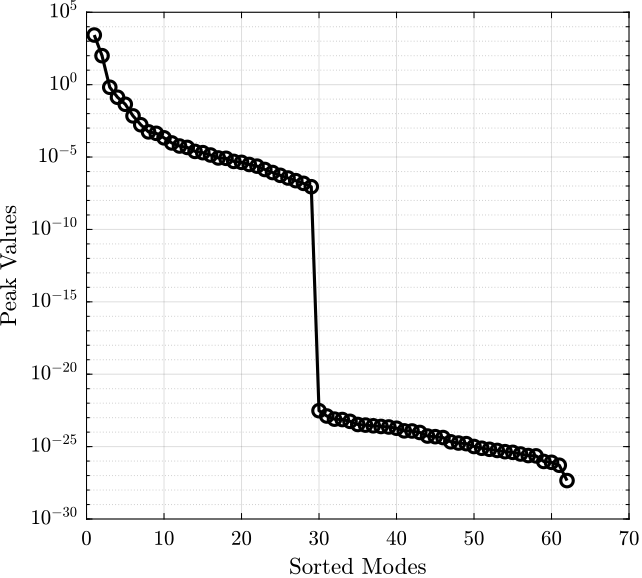
The modes are sorted by their peak gain. The obtained sorted peak gains for each mode are shown in figure fig:cant_beam_peak_gains_sorted.

dc_gain = abs(xn(i_input, :).*xn(i_output, :))./(2*pi*f0).^2;
peak_gain = dc_gain./xi;

[peak_gain_sort, index_sort] = sort(peak_gain, 'descend');

Model Reduction

Let’s keep only the first 10 sorted modes.

m_max = 10;

xn_s = xn(:, index_sort(1:m_max));
f0_s = f0(index_sort(1:m_max));
xi_s = xi(index_sort(1:m_max));

And we create the state space matrices.

Adiag = zeros(2*m_max,1);
Adiag(2:2:end) = -2*xi_s.*(2*pi*f0_s);

Adiagsup = zeros(2*m_max-1,1);
Adiagsup(1:2:end) = 1;

Adiaginf = zeros(2*m_max-1,1);
Adiaginf(1:2:end) = -(2*pi*f0_s).^2;

A = diag(Adiag) + diag(Adiagsup, 1) + diag(Adiaginf, -1);

B = zeros(2*m_max, length(i_input));

for i = 1:length(i_input)
    % Physical Coordinates
    Fp = zeros(n_nodes, 1);
    Fp(i_input(i)) = 1;

    B(2:2:end, i) = xn_s'*Fp;
end

C = zeros(length(i_output), 2*m_max);
C(:, 1:2:end) = xn_s(i_output, :);

D = zeros(length(i_output), length(i_input));

And finally the reduced State Space Model is created and compared with the full model in Figure fig:cant_beam_non_uniform_damp_reduced_dynamics.

G_p = ss(A, B, C, D);

MIMO System

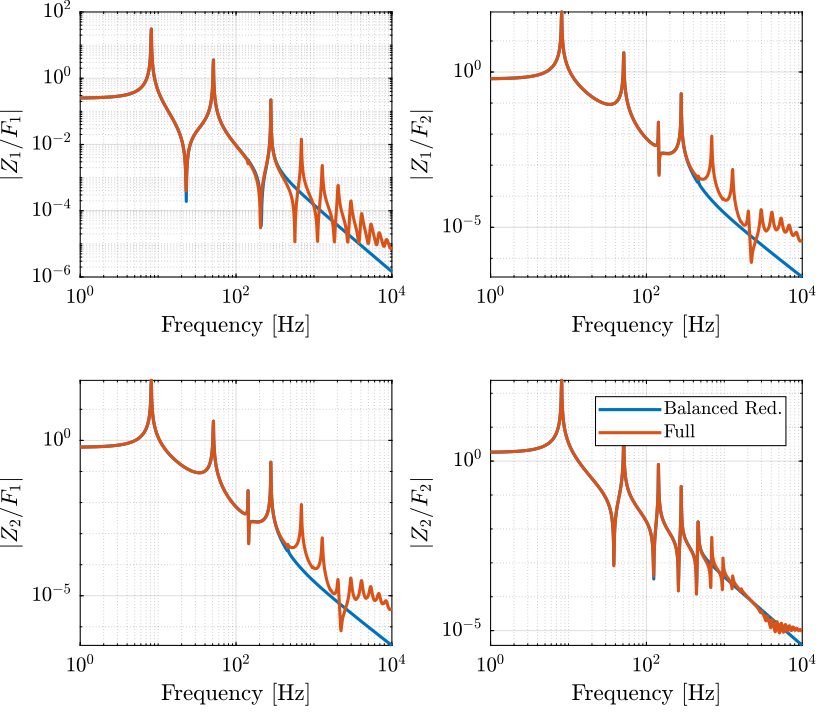
Introduction

When using multiple inputs and multiple outputs, one cannot simply choose the modes to keep based on their gains because this gain depends on the inputs and outputs chosen.

In such case, balancing reduction should be used.

Inputs and Outputs

Let’s choose two inputs and two outputs.

i_input = [14, 31];
i_output = [14, 31];

Full Model

The state space matrices are created by inspection.

Adiag = zeros(2*n_modes,1);
Adiag(2:2:end) = -2*xi.*(2*pi*f0);

Adiagsup = zeros(2*n_modes-1,1);
Adiagsup(1:2:end) = 1;

Adiaginf = zeros(2*n_modes-1,1);
Adiaginf(1:2:end) = -(2*pi*f0).^2;

A = diag(Adiag) + diag(Adiagsup, 1) + diag(Adiaginf, -1);

B = zeros(2*n_modes, length(i_input));

for i = 1:length(i_input)
    % Physical Coordinates
    Fp = zeros(n_nodes, 1);
    Fp(i_input(i)) = 1;

    B(2:2:end, i) = xn'*Fp;
end

C = zeros(length(i_output), 2*n_modes);
C(:, 1:2:end) = xn(i_output, :);

D = zeros(length(i_output), length(i_input));

And the State Space Model is created.

G_m = ss(A, B, C, D);

Balancing Reduction

First, we have to make sure that the rigid body mode is not included in the system (here it is not).

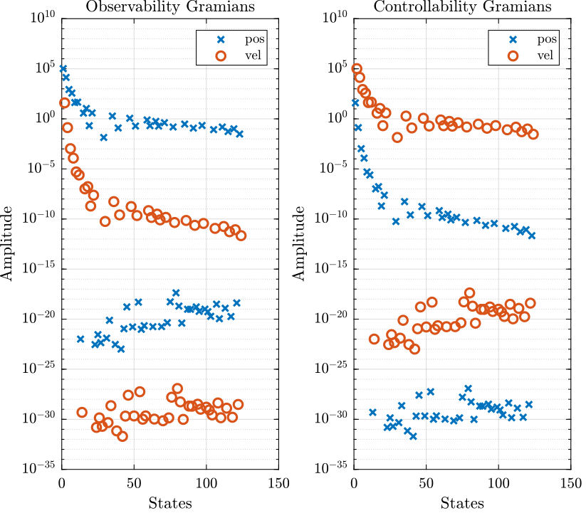
Then, we compute the controllability and observability gramians.

wc = gram(G_m, 'c');
wo = gram(G_m, 'o');

And we plot the diagonal terms of the controllability and observability gramians (Figure fig:cant_beam_gramians). The states representing the position and velocity are separated.

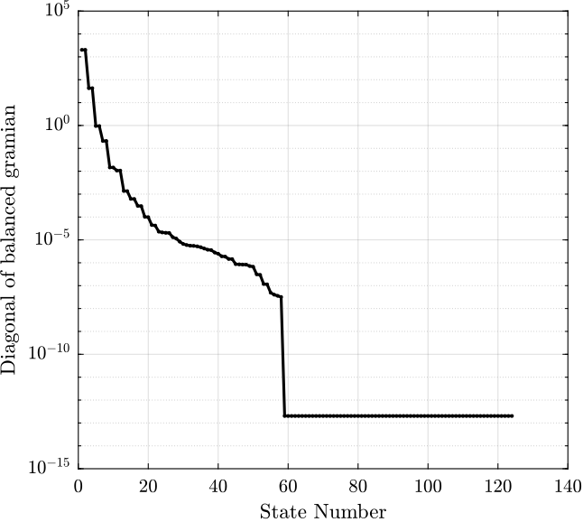
We use balreal to rank oscillatory states.

[SYSB,G] = BALREAL(SYS) computes a balanced state-space realization for the stable portion of the linear system SYS. For stable systems, SYSB is an equivalent realization for which the controllability and observability Gramians are equal and diagonal, their diagonal entries forming the vector G of Hankel singular values. Small entries in G indicate states that can be removed to simplify the model (use MODRED to reduce the model order).

[G_b, G, T, Ti] = balreal(G_m);

The diagonal values of the two gramians are shown in Figure fig:cant_beam_gramian_balanced.

Now we can choose the number of states to keep.

n_states_b = 10;

We now use modred to define reduced order oscillatory system using mathdc or truncate option.

MODRED Model simplification by state elimination.

RSYS = MODRED(SYS,ELIM) simplifies the state-space model SYS by discarding the states specified in the vector ELIM. The full state vector X is partitioned as X = [X1;X2] where Xr=X1 is the reduced state vector and X2 is discarded.

G_br = modred(G_b, n_states_b+1:size(A,1), 'truncate');

If needed, the rigid body mode should be added to the reduced system.

And other option is to specify the minimum value of the gramians diagonal elements for the modes to keep.

G_min = 1e-4;
G_br = modred(G_b, G<G_min, 'truncate');

The obtained reduced dynamics is shown in Figure fig:cant_beam_mimo_reduction.

Piezoelectric Stack Actuator / Sensor

Matlab Init

addpath('./src/');
addpath('examples/piezo_stack/');

Half Actuator / Half Sensor

Introduction

Import Mass Matrix, Stiffness Matrix, and Interface Nodes Coordinates

We first extract the stiffness and mass matrices.

K = extractMatrix('piezo_stack_half_K.txt');
M = extractMatrix('piezo_stack_half_M.txt');

Then, we extract the coordinates of the interface nodes.

[int_xyz, int_i, n_xyz, n_i, nodes] = extractNodes('piezo_stack_half.txt');

Total number of Nodes	1404
Number of interface Nodes	3
Number of Modes	186
Size of M and K matrices	204

Node Number	x [m]	y [m]	z [m]
1402.0	0.0	0.0	0.0
1403.0	0.035	0.0	0.0
1404.0	0.07	0.0	0.0

200000000.0	0	0	0	0	0	-200000000.0	0	0	0
0	10000000.0	0	0	0	200000.0	0	-10000000.0	0	0
0	0	10000000.0	8e-06	-200000.0	0	0	0	-10000000.0	4e-06
0	0	8e-06	1000.0	-4e-08	0	0	0	4e-06	-1000.0
0	0	-200000.0	-4e-08	6000.0	0	0	0	200000.0	-3e-08
0	200000.0	0	0	0	6000.0	0	-200000.0	0	0
-200000000.0	0	0	0	0	0	400000000.0	0	0	0
0	-10000000.0	0	0	0	-200000.0	0	30000000.0	0	0
0	0	-10000000.0	4e-06	200000.0	0	0	0	30000000.0	2e-05
0	0	4e-06	-1000.0	-3e-08	0	0	0	2e-05	2000.0

0.009	0	0	0	0	0	0.005	0	0	0
0	0.01	0	0	0	5e-05	0	0.004	0	0
0	0	0.01	-6e-16	-5e-05	0	0	0	0.004	-5e-16
0	0	-6e-16	2e-07	4e-18	0	0	0	-5e-16	8e-08
0	0	-5e-05	4e-18	3e-07	0	0	0	-3e-05	4e-18
0	5e-05	0	0	0	3e-07	0	3e-05	0	0
0.005	0	0	0	0	0	0.02	0	0	0
0	0.004	0	0	0	3e-05	0	0.02	0	0
0	0	0.004	-5e-16	-3e-05	0	0	0	0.02	-1e-15
0	0	-5e-16	8e-08	4e-18	0	0	0	-1e-15	3e-07

Using K, M and int_xyz, we can use the Reduced Order Flexible Solid simscape block.

Identification of the Dynamics

The flexible element is imported using the Reduced Order Flexible Solid simscape block.

To model the actuator, an Internal Force block is added between the first and second nodes. To model the sensors, a Relative Motion Sensor block is added between the second and the third nodes.

Two masses are fixed at the ends of the piezo-electric stack actuator.

We first set the mass to be zero.

m = 0;

The dynamics is identified from the applied force to the measured relative displacement.

%% Name of the Simulink File
mdl = 'piezo_stack';

%% Input/Output definition
clear io; io_i = 1;
io(io_i) = linio([mdl, '/F'], 1, 'openinput');  io_i = io_i + 1;
io(io_i) = linio([mdl, '/x'], 1, 'openoutput'); io_i = io_i + 1;

Gh = linearize(mdl, io);

Then, we add 1Kg of mass:

m = 1;

And the dynamics is identified.

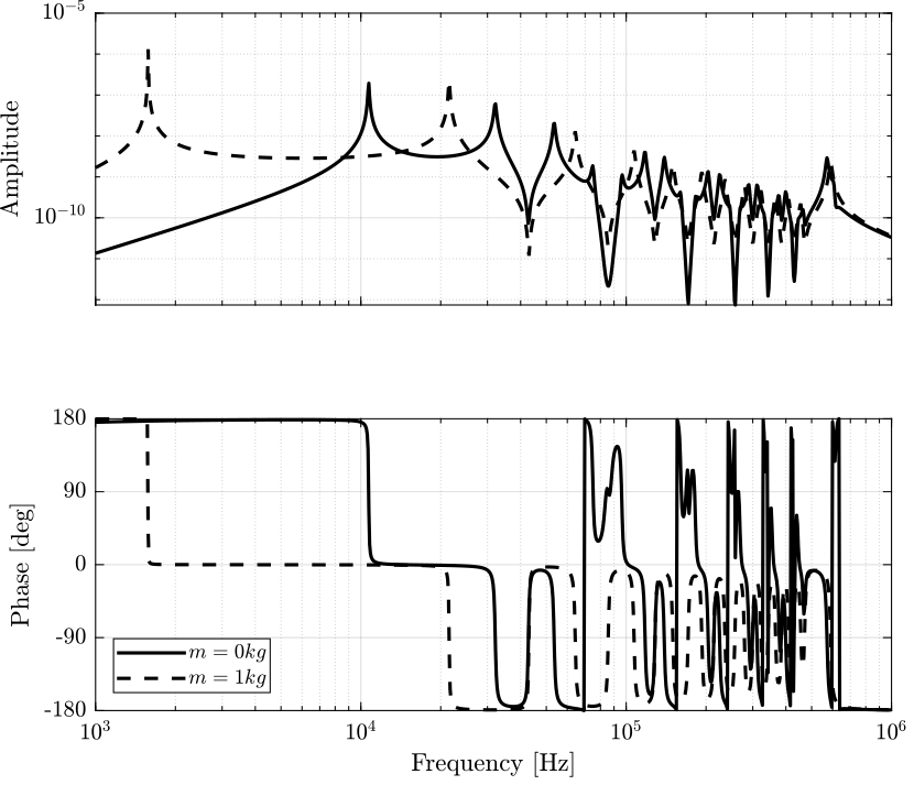
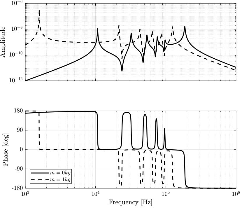
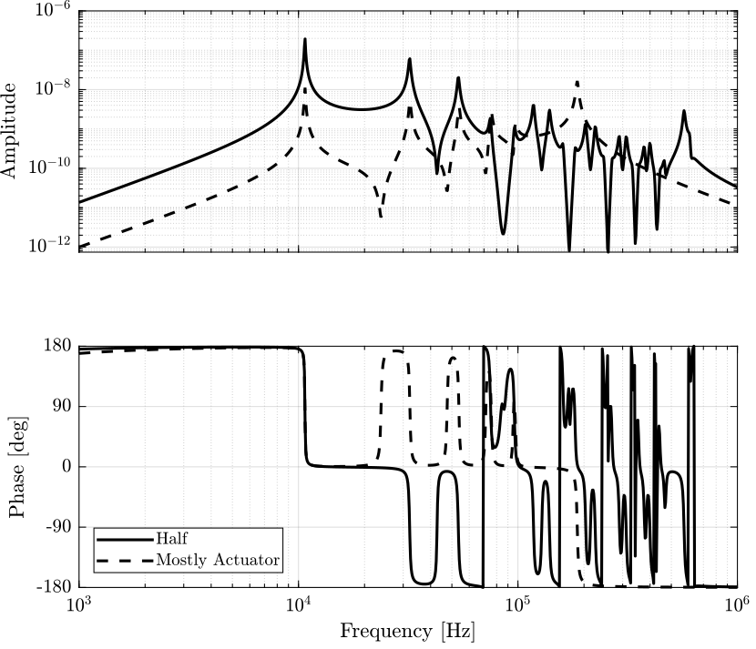
The two identified dynamics are compared in Figure fig:piezo_stack_half_frf.

Mostly Actuator / Barely Sensor

Introduction

Import Mass Matrix, Stiffness Matrix, and Interface Nodes Coordinates

We first extract the stiffness and mass matrices.

K = extractMatrix('piezo_stack_actuator_K.txt');
M = extractMatrix('piezo_stack_actuator_M.txt');

Then, we extract the coordinates of the interface nodes.

[int_xyz, int_i, n_xyz, n_i, nodes] = extractNodes('piezo_stack_actuator.txt');

Total number of Nodes	1401
Number of interface Nodes	3
Number of Modes	30
Size of M and K matrices	48

Node Number	x [m]	y [m]	z [m]
1.0	0.0	0.0	0.0
2.0	0.06	0.0	0.0
3.0	0.07	0.0	0.0

110000000.0	0.0	0.0	0.0	0.0	0.0	-110000000.0	0.0	0.0	0.0
0.0	2600000.0	0.0	1.3e-08	0.0	82000.0	0.0	-2600000.0	0.0	0.0
0.0	0.0	2600000.0	1.5e-05	-82000.0	0.0	0.0	0.0	-2600000.0	6.5e-06
0.0	1.3e-08	1.5e-05	610.0	-1.3e-07	6.3e-13	0.0	7.8e-13	6.5e-06	-610.0
0.0	0.0	-82000.0	-1.3e-07	3500.0	0.0	0.0	0.0	82000.0	-9.2e-08
0.0	82000.0	0.0	6.3e-13	0.0	3500.0	0.0	-82000.0	0.0	0.0
-110000000.0	0.0	0.0	0.0	0.0	0.0	1100000000.0	0.0	0.0	0.0
0.0	-2600000.0	0.0	7.8e-13	0.0	-82000.0	0.0	280000000.0	0.0	0.0
0.0	0.0	-2600000.0	6.5e-06	82000.0	0.0	0.0	0.0	280000000.0	1.7e-05
0.0	0.0	6.5e-06	-610.0	-9.2e-08	0.0	0.0	0.0	1.7e-05	6100.0

0.016	0.0	0.0	0.0	0.0	0.0	0.0082	0.0	0.0	0.0
0.0	0.018	0.0	-5.3e-21	0.0	0.00016	0.0	0.0064	0.0	0.0
0.0	0.0	0.018	-5.9e-15	-0.00016	0.0	0.0	0.0	0.0064	-5.2e-15
0.0	-5.3e-21	-5.9e-15	2.7e-07	7.7e-17	-4.7e-23	0.0	-1.9e-21	-5.2e-15	1.4e-07
0.0	0.0	-0.00016	7.7e-17	1.9e-06	0.0	0.0	0.0	-9.8e-05	7.2e-17
0.0	0.00016	0.0	-4.7e-23	0.0	1.9e-06	0.0	9.8e-05	0.0	0.0
0.0082	0.0	0.0	0.0	0.0	0.0	0.018	0.0	0.0	0.0
0.0	0.0064	0.0	-1.9e-21	0.0	9.8e-05	0.0	0.02	0.0	0.0
0.0	0.0	0.0064	-5.2e-15	-9.8e-05	0.0	0.0	0.0	0.02	-5.9e-15
0.0	0.0	-5.2e-15	1.4e-07	7.2e-17	0.0	0.0	0.0	-5.9e-15	3e-07

Using K, M and int_xyz, we can use the Reduced Order Flexible Solid simscape block.

Identification of the Dynamics

The flexible element is imported using the Reduced Order Flexible Solid simscape block.

To model the actuator, an Internal Force block is added between the first and second nodes. To model the sensors, a Relative Motion Sensor block is added between the second and the third nodes.

Two masses are fixed at the ends of the piezo-electric stack actuator.

We first set the mass to be zero.

m = 0;

The dynamics is identified from the applied force to the measured relative displacement.

%% Name of the Simulink File
mdl = 'piezo_stack';

%% Input/Output definition
clear io; io_i = 1;
io(io_i) = linio([mdl, '/F'], 1, 'openinput');  io_i = io_i + 1;
io(io_i) = linio([mdl, '/x'], 1, 'openoutput'); io_i = io_i + 1;

Ga = linearize(mdl, io);

Then, we add 1Kg of mass:

m = 1;

And the dynamics is identified.

With Mode Modes

K = extractMatrix('piezo_stack_actuator_bis_K.txt');
M = extractMatrix('piezo_stack_actuator_bis_M.txt');
[int_xyz, int_i, n_xyz, n_i, nodes] = extractNodes('piezo_stack_actuator_bis.txt');

Total number of Nodes	1401
Number of interface Nodes	3
Number of Modes	120
Size of M and K matrices	138

m = 0;

%% Name of the Simulink File
mdl = 'piezo_stack';

%% Input/Output definition
clear io; io_i = 1;
io(io_i) = linio([mdl, '/F'], 1, 'openinput');  io_i = io_i + 1;
io(io_i) = linio([mdl, '/x'], 1, 'openoutput'); io_i = io_i + 1;

Gb = linearize(mdl, io);

m = 1;

Comparison

Amplified Piezoelectric Actuator

Matlab Init

addpath('./src/');
addpath('examples/piezo_amplified/');

Import Mass Matrix, Stiffness Matrix, and Interface Nodes Coordinates

We first extract the stiffness and mass matrices.

K = extractMatrix('piezo_amplified_K.txt');
M = extractMatrix('piezo_amplified_M.txt');

Then, we extract the coordinates of the interface nodes.

[int_xyz, int_i, n_xyz, n_i, nodes] = extractNodes('piezo_amplified.txt');

Total number of Nodes	14
Number of interface Nodes	13
Number of Modes	30
Size of M and K matrices	108

Node i	Node Number	x [m]	y [m]
1.0	76423.0	0.0	0.03
2.0	76429.0	0.0	-0.03
3.0	76430.0	-0.035	0.0
4.0	76431.0	0.028	0.0
5.0	76432.0	0.021	0.0
6.0	76433.0	0.014	0.0
7.0	76434.0	0.007	0.0
8.0	76435.0	0.0	0.0
9.0	76436.0	-0.007	0.0
10.0	76437.0	-0.014	0.0
11.0	76438.0	-0.021	0.0
12.0	76439.0	-0.028	0.0
13.0	76440.0	0.035	0.0

200000000.0	30000.0	-1000.0	-4	-70.0	-80000.0	100000000.0	3000.0	1000.0	-20.0
30000.0	80000000.0	-1000.0	60.0	30.0	-100.0	-1000.0	-40000000.0	3000.0	80.0
-1000.0	-1000.0	30000000.0	-600000.0	20.0	6	4000.0	1000.0	10000000.0	100000.0
-4	60.0	-600000.0	20000.0	-0.6	-0.02	-100.0	6	-100000.0	-1000.0
-70.0	30.0	20.0	-0.6	30000.0	0.2	-50.0	-200.0	6	0.07
-80000.0	-100.0	6	-0.02	0.2	3000.0	20000.0	30.0	5	0.04
100000000.0	-1000.0	4000.0	-100.0	-50.0	20000.0	200000000.0	20000.0	5000.0	-30.0
3000.0	-40000000.0	1000.0	6	-200.0	30.0	20000.0	80000000.0	7000.0	20.0
1000.0	3000.0	10000000.0	-100000.0	6	5	5000.0	7000.0	30000000.0	600000.0
-20.0	80.0	100000.0	-1000.0	0.07	0.04	-30.0	20.0	600000.0	20000.0

0.04	2e-06	-1e-06	4e-09	2e-08	0.0002	-0.01	-1e-06	1e-06	7e-09
2e-06	0.02	2e-06	-2e-08	-1e-08	5e-08	-2e-08	0.002	-2e-06	-2e-08
-1e-06	2e-06	0.03	-0.0001	2e-08	-5e-10	-3e-06	-3e-07	-0.003	-2e-05
4e-09	-2e-08	-0.0001	1e-06	-2e-10	-1e-10	2e-08	2e-10	2e-05	2e-07
2e-08	-1e-08	2e-08	-2e-10	2e-06	-4e-10	3e-08	4e-08	-3e-09	5e-11
0.0002	5e-08	-5e-10	-1e-10	-4e-10	2e-06	-2e-05	-1e-08	-7e-10	-7e-12
-0.01	-2e-08	-3e-06	2e-08	3e-08	-2e-05	0.04	2e-07	2e-06	7e-09
-1e-06	0.002	-3e-07	2e-10	4e-08	-1e-08	2e-07	0.02	-4e-07	2e-10
1e-06	-2e-06	-0.003	2e-05	-3e-09	-7e-10	2e-06	-4e-07	0.03	0.0001
7e-09	-2e-08	-2e-05	2e-07	5e-11	-7e-12	7e-09	2e-10	0.0001	1e-06

Using K, M and int_xyz, we can use the Reduced Order Flexible Solid simscape block.

Identification of the Dynamics

The flexible element is imported using the Reduced Order Flexible Solid simscape block.

To model the actuator, an Internal Force block is added between the first and second nodes. To model the sensors, a Relative Motion Sensor block is added between the second and the third nodes.

Two masses are fixed at the ends of the piezo-electric stack actuator.

We first set the mass to be zero.

m = 0;

The dynamics is identified from the applied force to the measured relative displacement.

%% Name of the Simulink File
mdl = 'piezo_amplified';

%% Input/Output definition
clear io; io_i = 1;
io(io_i) = linio([mdl, '/F'], 1, 'openinput');  io_i = io_i + 1;
io(io_i) = linio([mdl, '/y'], 1, 'openoutput'); io_i = io_i + 1;

Gh = linearize(mdl, io);

Then, we add 10Kg of mass:

m = 10;

And the dynamics is identified.

The two identified dynamics are compared in Figure fig:piezo_stack_half_frf.

Force Sensor

m = 0;

Comparison with Ansys

m = 0;

%% Name of the Simulink File
mdl = 'piezo_amplified';

%% Input/Output definition
clear io; io_i = 1;
io(io_i) = linio([mdl, '/F'], 1, 'openinput');  io_i = io_i + 1;
io(io_i) = linio([mdl, '/y'], 1, 'openoutput'); io_i = io_i + 1;

Gh = linearize(mdl, io);

a = tdfread('FEA-Response-Top.txt', ',');

Functions

<sec:functions>

`extractMatrix`: Extract Mass/Stiffness matrices

<sec:extractMatrix>

This Matlab function is accessible here.

Function description

function [M] = extractMatrix(filename)
% extractMatrix -
%
% Syntax: [M] = extractMatrix(filename)
%
% Inputs:
%    - filename - relative or absolute path of the file that contains the Matrix
%
% Outputs:
%    - M - Matrix that is contained in the file

Optional Parameters

arguments
    filename
end

Read the file

str = fileread(filename);

Extract the Matrix

str = regexprep(str,'\s+','');

parts = regexp(str, '\[(?<row>\d+),(?<col>\d+)\]:(?<val>[^\[]+)', 'names');

Get the number of column and rows

row = cellfun(@str2double, {parts.row}, 'UniformOutput', true);

col = cellfun(@str2double, {parts.col}, 'UniformOutput', true);

Get the values of the matrix

val = cellfun(@str2double, {parts.val}, 'UniformOutput', true);

Get the size of the matrix

sz = [max(row), max(col)];

Create the Matrix with the correct size

M = zeros(sz);

Get matrix position corresponding to the values.

ix = sub2ind(sz, row, col);

Finally, data are assigned.

M(ix)= val;

`extractNodes`: Extract Nodes positions and Interfaces DoFs

<sec:extractNodes>

This Matlab function is accessible here.

Function description

function [int_xyz, int_i, n_xyz, n_i, nodes] = extractNodes(filename)
% extractNodes -
%
% Syntax: [n_xyz, nodes] = extractNodes(filename)
%
% Inputs:
%    - filename - relative or absolute path of the file that contains the Matrix
%
% Outputs:
%    - n_xyz -
%    - nodes - table containing the node numbers and corresponding dof of the interfaced DoFs

Optional Parameters

arguments
    filename
end

Read the file

fid = fopen(filename,'rt');

if fid == -1
    error('Error opening the file');
end

Extract Nodes

n_xyz = []; % Contains nodes coordinates
n_i = []; % Contains nodes indices

n_num = []; % Contains node numbers
n_dof = {}; % Contains node directions

while 1
    % Read a line
    nextline = fgetl(fid);

    % End of the file
    if ~isstr(nextline), break, end

    % Line just before the list of nodes coordinates
    if contains(nextline, 'NODE') && ...
            contains(nextline, 'X') && ...
            contains(nextline, 'Y') && ...
            contains(nextline, 'Z')

        while 1
            nextline = fgetl(fid);

            if nextline < 0, break, end

            c = sscanf(nextline, ' %f');

            if isempty(c), break, end

            n_xyz = [n_xyz; c(2:4)'];
            n_i = [n_i; c(1)];
        end
    end

    if nextline < 0, break, end

    % Line just before the list of node DOF
  if contains(nextline, 'NODE') && ...
         contains(nextline, 'LABEL')

        while 1
            nextline = fgetl(fid);

            if nextline < 0, break, end

            c = sscanf(nextline, ' %d %s');

            if isempty(c), break, end

            n_num = [n_num; c(1)];

            n_dof{length(n_dof)+1} = char(c(2:end)');
        end

        nodes = table(n_num, string(n_dof'), 'VariableNames', {'node_i', 'node_dof'});
    end

    if nextline < 0, break, end
end

Close the file

fclose(fid);

Get XYZ coordinates of the interface nodes

int_i = unique(nodes.('node_i')); % indices of interface nodes

% Extract XYZ coordinates of only the interface nodes
if length(n_xyz) > 0 && length(n_i) > 0
    int_xyz = n_xyz(logical(sum(n_i.*ones(1, length(int_i)) == int_i', 2)), :);
else
    int_xyz = n_xyz;
end

`extractEigs`: Extract Eigen Values and Eigen Vectors

<sec:extractEigs>

This Matlab function is accessible here.

Function description

function [zm, w] = extractEigs(filename, args)
% extractEigs -
%
% Syntax: [zm, w] = extractEigs(filename, args)
%
% Inputs:
%    - filename - relative or absolute path of the file that contains the eigenvectors and eigenvalues
%    - args - Optional parameters:
%        - dirs - [6 x 1] - ones(6,1) (default)
%                          - Vectors with 0 and 1 identifying directions to include in the modal matrix
%                          - This corresponds to [Ux, Uy, Uz, Rx, Ry, Rz]
%        - soft - 'ansys' (default) - Software used for the FEM
%
% Outputs:
%    - zm - [(n x dofs) x m] - Modal Matrix containing the eigenvectors
%                            - zm(1:n, i) corresponds to the eigenvector for mode i and for first dir considered
%                            - zm((n-1)*j+1:n*j, i) corresponds to the eigenvector for i'th mode and for j'th dir considered
%    - w  - [m x 1] - Eigenvalues [Hz]

Optional Parameters

arguments
    filename
    args.dirs (6,1) double {mustBeNumericOrLogical}            = ones(6,1)
    args.soft       char   {mustBeMember(args.soft,{'ansys'})} = 'ansys'
end

Open the file

fid = fopen(filename,'rt');

if fid == -1
    error('Error opening the file');
end

Extract Eigenvalues - Ansys

if strcmp(args.soft, 'ansys')
    w = [];
    zm = [];

    while 1
        % Read a line
        nextline = fgetl(fid);

        % End of the file
        if ~isstr(nextline), break, end

        % Lines containing the mode numbers
        if contains(nextline, ' LOAD STEP=') && ...
                contains(nextline, 'SUBSTEP=') && ...
                ~contains(nextline, 'CUM')
            mode_num = sscanf(nextline, ' LOAD STEP= %*f  SUBSTEP= %f ');
        end

        % Lines containing the frequency of the modes
        if contains(nextline, 'FREQ=')
            w = [w, sscanf(nextline, ' FREQ= %f LOAD CASE= %*f')];
        end

        % Start of the eigenvectors
        if contains(nextline, 'ROTZ')
            zmi = [];

            % Read the eigenvectors for each of the nodes
            while 1
                nextline = fgetl(fid);
                c = sscanf(nextline, ' %f');
                if isempty(c), break, end
                zmi = [zmi; c(2:end)'];
            end

            zm (:, :, mode_num) = zmi;
        end
    end

    zm = reshape(zm(:, logical([0; args.dirs]), :), size(zm, 1)*sum(args.dirs), size(zm, 3));
end

Close the file

fclose(fid);

`normalizeEigs`: Normalize Eigen Vectors

<sec:normalizeEigs>

This Matlab function is accessible here.

Function description

function [zn] = normalizeEigs(zm, args)
% normalizeEigs - Normalize the eigenvectors
%
% Syntax: [zn] = normalizeEigs(zm, args)
%
% Inputs:
%    - zm - Modal Matrix
%    - args - Optional parameters:
%        - method - 'mass' (default), 'unity' - Method used to normalize the eigenvectors
%
% Outputs:
%    - zn - Normalized Modal Matrix

Optional Parameters

arguments
    zm
    args.m      double {mustBeNumeric} = 0
    args.method char   {mustBeMember(args.method,{'mass', 'unity'})} = 'mass'
end

Normalize the Eigen Vectors - Mass Method

if strcmp(args.method, 'mass')
    if size(args.m) ~= [size(zm,1), size(zm,1)]
        error('The provided Mass matrix has not a compatible size with the Modal Matrix')
    end
 
    zn = zeros(size(zm));
    for i = 1:size(zm,2)
        zn(:,i) = zm(:,i)/sqrt(zm(:,i)'*args.m*zm(:,i));
    end
end

Normalize the Eigen Vectors - Unity Method

if strcmp(args.method, 'unity')
  zn = zm./max(zm);
end

`reductionInOut`: Reduce the Modal matrix to some nodes

<sec:reductionInOut>

This Matlab function is accessible here.

Function description

function [zr] = reductionInOut(zn, i_inputs, i_outputs)
% reductionInOut - Reduce the Modal Matrix to only specified nodes corresponding to Inputs and Ouputs
%
% Syntax: [zr] = reductionInOut(zn, i_inputs, i_outputs)
%
% Inputs:
%    - zn        - Normalized Modal Matrix
%    - i_inputs  - Node indices corresponding to inputs
%    - i_outputs - Node indices corresponding to inputs
%
% Outputs:
%    - zr - Reduced Normalized Modal Matrix

Arguments

arguments
    zn
    i_inputs  {mustBeInteger} = 0
    i_outputs {mustBeInteger} = 0
end

Size Reduction

zr = zn([i_inputs, i_outputs], :);

`computeModalDamping` - Compute the Damping

<sec:computeModalDaping>

This Matlab function is accessible here.

Function description

function [xi] = computeModalDaping(z, w, args)
% computeModalDaping -
%
% Syntax: [xi] = computeModalDaping(z, w, args)
%
% Inputs:
%    - z, w, args -
%
% Outputs:
%    - xi -

Arguments

arguments
end

`sortModes` - Sort Modes

<sec:sortModes>

This Matlab function is accessible here.

Function description

function [modes_i] = sortModes(z, w, xi, args)
% sortModes -
%
% Syntax: [modes_i] = sortModes(z, w, xi, args)
%
% Inputs:
%    - z, w, xi, args -
%
% Outputs:
%    - modes_i -

end

Arguments

arguments
end

`reduceModes` - Get Modes numbers for the reduced model

<sec:reduceModes>

This Matlab function is accessible here.

Function description

function [modes_i] = reduceModes(z, w, xi, args)
% reduceModes -
%
% Syntax: [modes_i] = reduceModes(z, w, xi, args)
%
% Inputs:
%    - z, w, xi, args -
%
% Outputs:
%    - modes_i -

Arguments

arguments
end

`createStateSpaceModel` - Create the Reduced State Space Model

<sec:createStateSpaceModel>

This Matlab function is accessible here.

Function description

function [G] = createStateSpaceModel(z, w, xi, modes_i)
% createStateSpaceModel -
%
% Syntax: [G] = createStateSpaceModel(z, w, xi, modes_i)
%
% Inputs:
%    - z, w, xi, modes_i -
%
% Outputs:
%    - G -

Arguments

arguments
end

Bibliography

bibliographystyle:unsrt bibliography:ref.bib

Finite Element Model - Matlab Toolbox

Introduction

Import Flexible Elements in Simscape using Component Mode Synthesis in Ansys

Introduction

Matlab Init

Import Mass Matrix, Stiffness Matrix, and Interface Nodes Coordinates

Identification of the Dynamics

Low Order Dynamical Model from a Finite Element Model

Introduction

Matlab Init

Extract Eigenvalues and Eigenvectors

Define Physical Inputs and Outputs

Define Damping

All Modes Included in the Model

Simple mode truncation

Modes sorted by their DC gain

Comparison

Effect of the Individual Modes

Non-Uniform Damping

Definition of the Damping

State Space Model

Obtained Dynamics

Sort Modes based on their peak gain

Model Reduction

MIMO System

Introduction

Inputs and Outputs

Full Model

Balancing Reduction

Piezoelectric Stack Actuator / Sensor

Matlab Init

Half Actuator / Half Sensor

Introduction

Import Mass Matrix, Stiffness Matrix, and Interface Nodes Coordinates

Identification of the Dynamics

Mostly Actuator / Barely Sensor

Introduction

Import Mass Matrix, Stiffness Matrix, and Interface Nodes Coordinates

Identification of the Dynamics

With Mode Modes

Comparison

Amplified Piezoelectric Actuator

Matlab Init

Import Mass Matrix, Stiffness Matrix, and Interface Nodes Coordinates

Identification of the Dynamics

Force Sensor

Comparison with Ansys

Functions

extractMatrix: Extract Mass/Stiffness matrices

Function description

Optional Parameters

Read the file

Extract the Matrix

extractNodes: Extract Nodes positions and Interfaces DoFs

Function description

Optional Parameters

Read the file

Extract Nodes

Close the file

Get XYZ coordinates of the interface nodes

extractEigs: Extract Eigen Values and Eigen Vectors

Function description

Optional Parameters

Open the file

Extract Eigenvalues - Ansys

Close the file

normalizeEigs: Normalize Eigen Vectors

Function description

Optional Parameters

Normalize the Eigen Vectors - Mass Method

Normalize the Eigen Vectors - Unity Method

reductionInOut: Reduce the Modal matrix to some nodes

Function description

Arguments

Size Reduction

computeModalDamping - Compute the Damping

Function description

Arguments

sortModes - Sort Modes

Function description

`extractMatrix`: Extract Mass/Stiffness matrices

`extractNodes`: Extract Nodes positions and Interfaces DoFs

`extractEigs`: Extract Eigen Values and Eigen Vectors

`normalizeEigs`: Normalize Eigen Vectors

`reductionInOut`: Reduce the Modal matrix to some nodes

`computeModalDamping` - Compute the Damping

`sortModes` - Sort Modes

`reduceModes` - Get Modes numbers for the reduced model

`createStateSpaceModel` - Create the Reduced State Space Model