Data visualization can help programmers and scientists identify trends in their data and efficiently communicate these results with their peers. Modern C++ is being used for a variety of scientific applications, and this environment can benefit considerably from graphics libraries that attend the typical design goals toward scientific data visualization. Besides the option of exporting results to other environments, the customary alternatives in C++ are either non-dedicated libraries that depend on existing user interfaces or bindings to other languages. Matplot++ is a graphics library for data visualization that provides interactive plotting, means for exporting plots in high-quality formats for scientific publications, a compact syntax consistent with similar libraries, dozens of plot categories with specialized algorithms, multiple coding styles, and supports generic backends.


![]()
![]()


The examples assume we are in the matplot namespace. Use these examples to understand how to quickly use the library for data visualization. If you are interested in understanding how the library works, you can later read the details in the complete article.
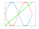
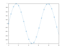
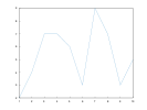
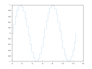
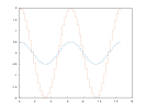
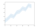
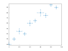
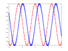
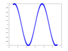
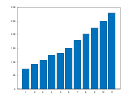
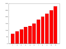
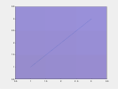
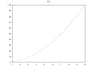
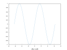
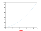
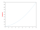
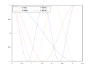
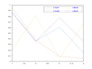
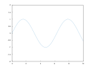
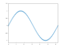
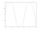
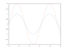
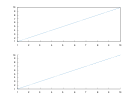
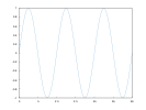
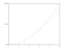
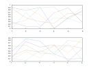
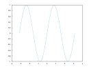
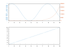
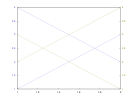
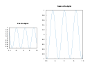
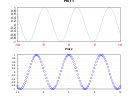
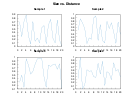
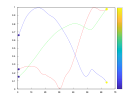
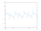
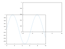
- Line Plot
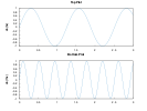
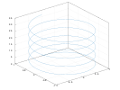
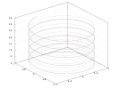
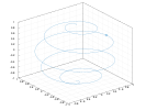
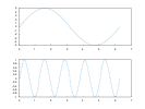
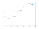
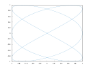
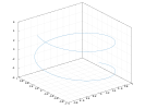
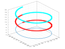
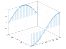
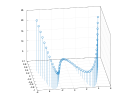
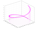
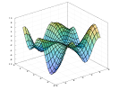
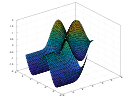
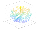
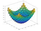
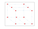
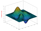
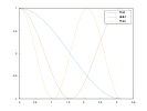
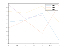
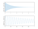
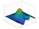
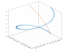
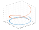
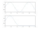
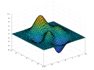
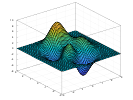
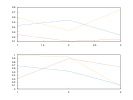
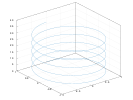
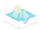
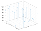
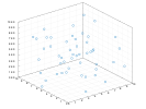
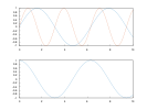
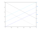
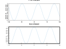
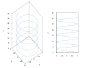
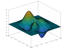
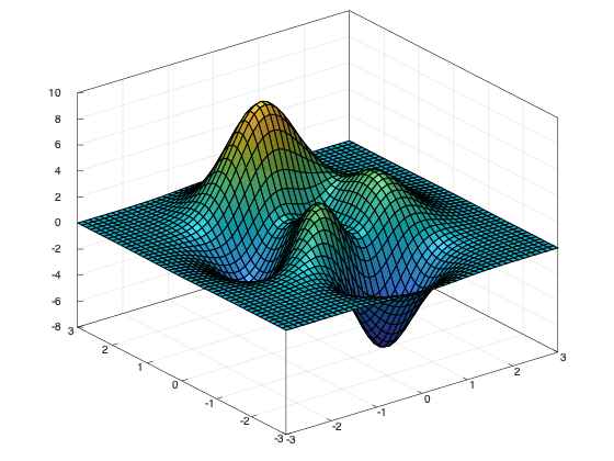
- Line Plot 3D
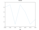
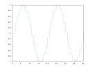
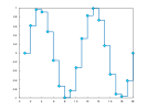
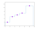
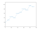
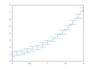
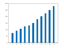
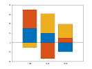
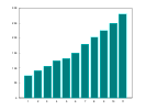
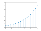
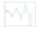
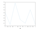
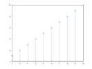
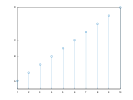
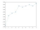
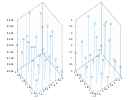
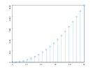
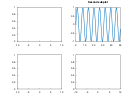
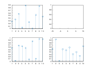
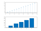
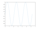
- Stairs
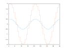
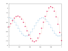
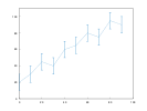
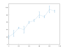
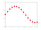
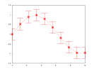
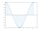
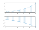
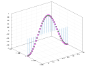
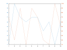
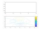
- Error Bars
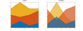
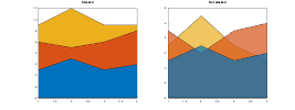
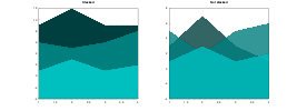
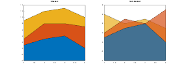
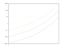
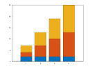
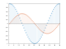
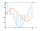
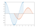
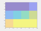
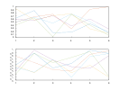
- Area
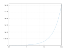
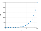
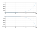
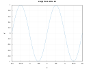
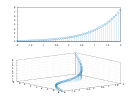
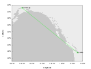
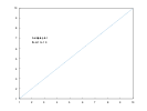
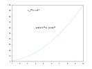
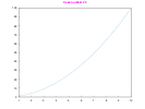
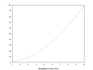
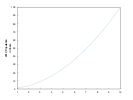
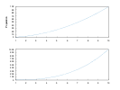
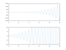
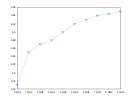
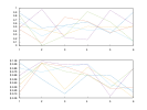
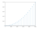
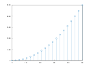
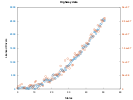
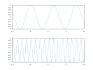
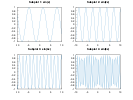
- Loglog Plot
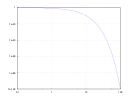
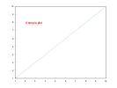
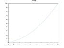
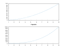
- Semilogx Plot
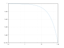
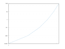
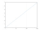
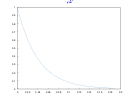
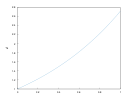
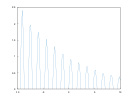
- Semilogy Plot
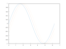
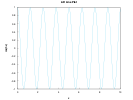
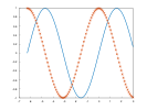
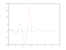
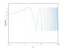
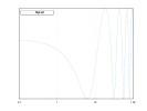
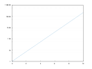
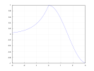
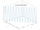
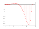
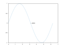
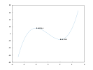
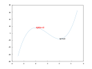
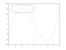
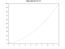
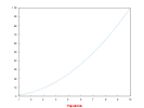
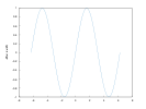
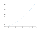
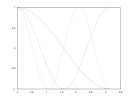
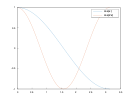
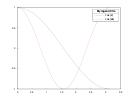
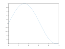
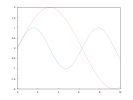
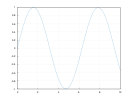
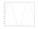
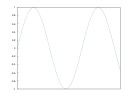
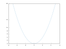
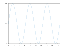
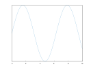
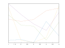
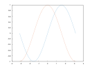
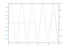
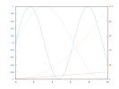
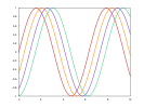
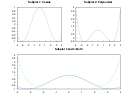
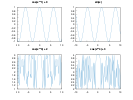
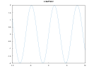
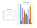
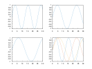
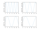
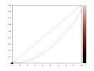
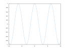
- Function Plot
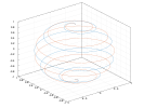
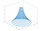
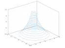
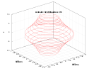
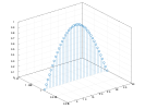
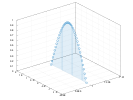
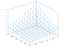
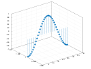
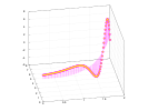
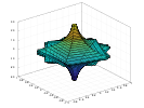
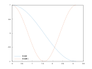
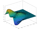
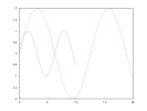
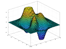
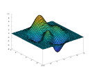
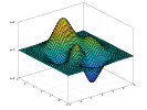
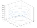
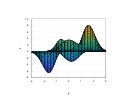
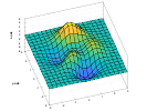
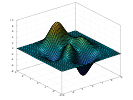
- Function Plot 3D
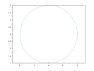
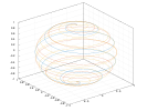
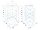
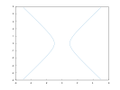
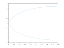
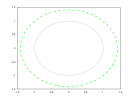
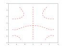
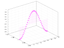
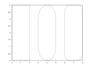
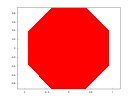
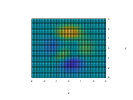
- Implicit function
plot(x,y); 
Where x and y are are any value ranges.
More examples:
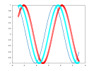
Setters return a reference to *this to allow method chaining:
plot(x,y)->line_width(2).color("red");The examples use free-standing functions to create plots. You can also use a object-oriented style for plots. We discuss these coding styles in the Section Coding Styles.
plot3(x,y);
More examples:
With method chaining:
plot3(x,y)->line_width(2).color("red");stairs(x,y);
More examples:
The stair object renders the line with stairs between data points to denote discrete data.
errorbar(x,y,err);
More examples:
The error bar object includes extra lines to represent error around data points. Log plots are utility functions that adjust the x or y axes to a logarithmic scale.
area(Y);
More examples:
loglog(x,y);
More examples:
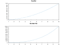
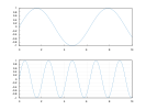
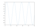
semilogx(x,y);
semilogy(x,y);
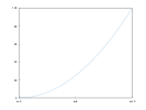
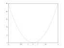
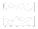
fplot(fx);
More examples:
Instead of storing data points, the objects function line and string function store a function as a lambda function or as a string with an expression. These objects use lazy evaluation to generate absolute data points. The data is generated only when the draw function is called.
fplot(fxy);
More examples:
fplot(fxy);
More examples:
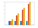
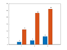
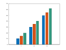
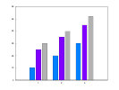
- Histogram
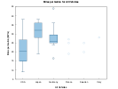
- Boxplot
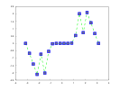
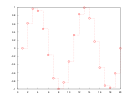
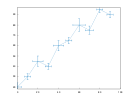
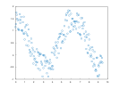
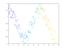
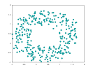
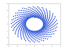
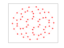
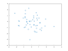
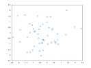
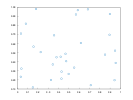
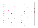
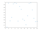
- Scatter Plot
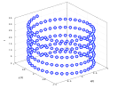
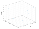
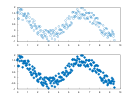
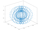
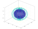
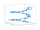
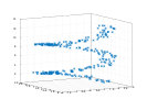
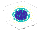
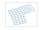
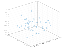
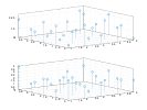
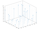
- Scatter Plot 3D
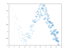
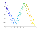
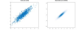
- Binscatter
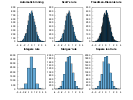
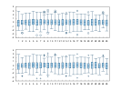
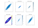
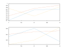
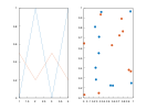
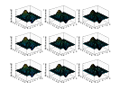
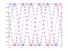
- Plot Matrix
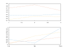
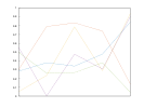
- Parallel Coordinates
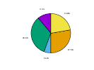
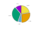
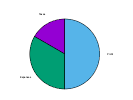
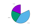
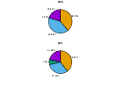
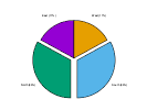
- Pie Chart
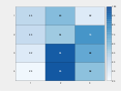
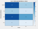
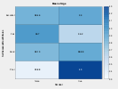
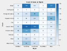
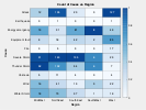
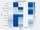
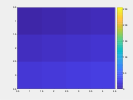
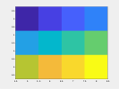
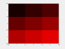
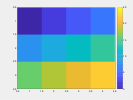
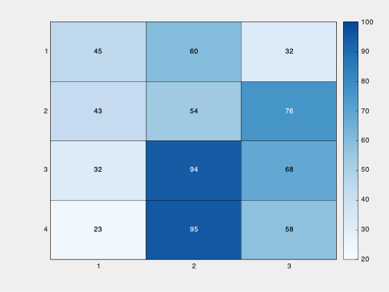
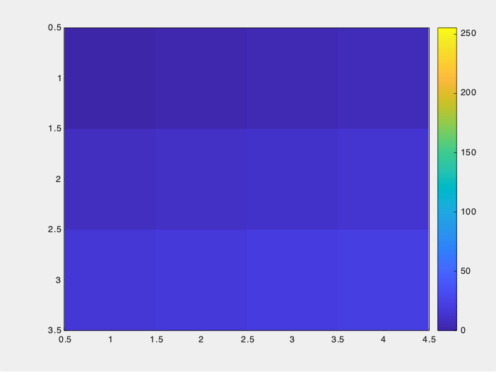
- Heatmap
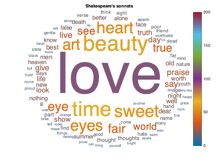
- Word Cloud
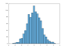
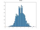
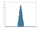
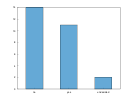
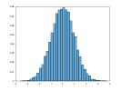
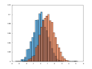
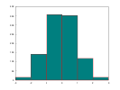
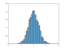
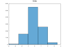
hist(data);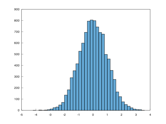
More examples:
The histogram object creates the histogram edges and bins when the draw function is called for the first time with lazy evaluation. Lazy evaluation avoids calculating edges unnecessarily in case the user changes the object parameters before calling draw. This object includes several algorithms for automatically delimiting the edges and bins for the histograms.
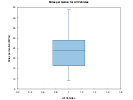
boxplot(data);
More examples:
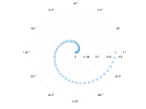
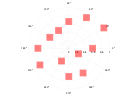
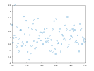
scatter(x,y);
More examples:
Scatter plots also depend on the line object. As the line object can represent lines with markers, the scatter function simply creates markers without the lines.
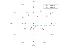
scatter(x,y,z);
More examples:
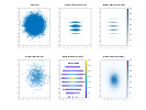
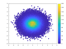
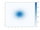
binscatter(x,y);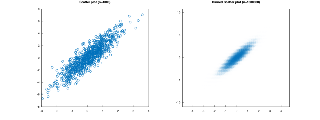
More examples:
Binned scatter plots use variations of the histogram algorithms of the previous section as an extra step to place all the data into two-dimensional bins that can be represented with varying colors or sizes. This is useful when there are so many data points that a scatter plot would be impractical for visualizing the data.
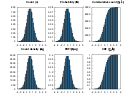
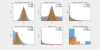
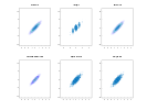
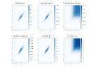
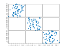
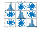
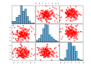
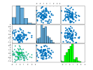
plotmatrix(X);
More examples:
The Plot Matrix subcategory is a combination of histograms and scatter plots. It creates a matrix of axes objects on the figure and creates a scatter plot for each pair of data sets.

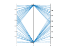
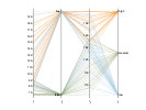
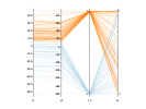
More examples:
The function parallelplot creates a plot with Parallel Coordinates. In this type of plot, a parallel lines object stores an arbitrary set of axis objects to represent multi-dimensional data.

More examples:
More examples:
More examples:
Word clouds are generated from text or pairs of words and their frequency. After attributing a size proportional to each word frequency, the algorithm to position the labels iterates words from the largest to the smallest. For each word, it spins the word in polar coordinates converted to Cartesian coordinates until it does not overlap with any other word.
By default, the colors and the sizes depend on the word frequencies. We can customize the colors by passing a third parameter to the wordcloud function.
More examples:

More examples:
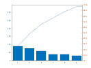
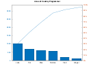
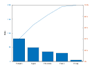
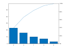
Pareto Charts are a type of chart that uses both
If you need Pareto fronts rather than Pareto charts, we refer to Scatter Plots for two-dimensional fronts, Plot matrices for three-dimensional fronts, or Parallel Coordinate Plots for many-objective fronts. These plot subcategories are described in Section Data Distribution. If you also need a tool to calculate these fronts efficiently, we refer to the Pareto Front Library.

More examples:

More examples:

More examples:
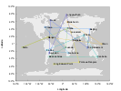
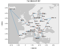
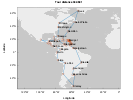
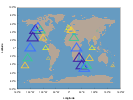
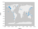
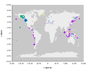
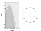
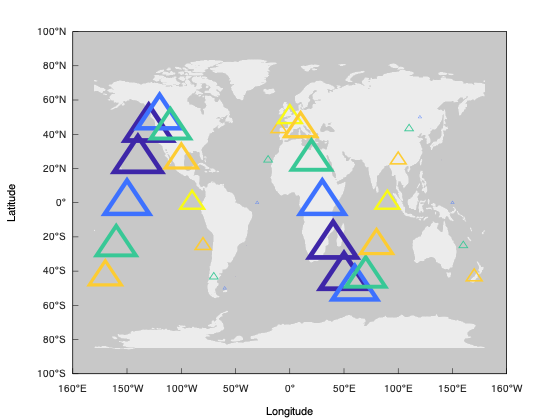
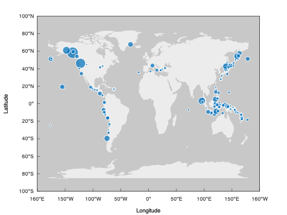
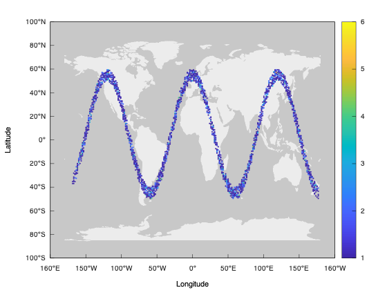
For the first geography plot, Matplot++ calls geoplot(), which creates a filled polygon with the world map. This first plot receives the tag "map" so that subsequent geography plots recognize there is no need to recreate this world map.
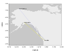
The data for the world map comes from Natural Earth. They provide data at 1:10m, 1:50m, and 1:110m scales. The geoplot function will initially use the data at the 1:110m scales. The geolimits function can be used to update the axis limits for geography plots. The difference between the usual functions for adjusting axis limits (xlim and ylim) and geolimits is that the latter will also update the map resolution according to the new limits for the
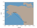
The geolimits function will query the figure size and, depending on the new limits for the axes, update the map to the 1:10m, or 1:50m scales if needed. Because it would be very inefficient to render the whole world map at a 1:10m or 1:50m scale only to display a region of this map, the geolimits function also crops the data pertinent to the new region being displayed.
Note that this does not only involve removing data points outside the new limits but it also needs to create new data points on the correct borders to create new polygons coherent with the map entry points in the region. For this reason, the algorithm needs to track all submaps represented as closed polygons in the original world map. If submaps are completely inside or outside the new ranges, we can respectively include or dismiss the data points. However, if the submap is only partially inside the new limits, to generate the correct borders for the polygons, we need to track all points outside the limits to classify the directions of these points outside the limits. We do that by only including points that change quadrants around the new limits so that the map entry points create polygons that look like they would if the complete world map were still being rendered outside these new limits.
If the you are not interested in geographic plots, the build script includes an option to remove the high-resolution maps at 1:10m and 1:50m scales from the library. In this case, the library will always use the map at a 1:110m scale no matter the axis limits.
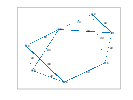
The function world_cities returns a list of major world cities. Its parameters define the minimum distances between cities in the greedy_tsp function is a naive greedy algorithm to find a route between these cities as a Traveling Salesman Problem (TSP). We use the geoplot function to draw this route. Note that we use method chaining to define some further plot properties. Finally, the text function includes the city names in the map.
More examples:
More examples:

More examples:
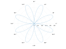
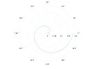
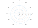
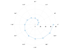
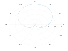
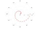
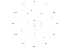
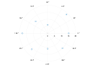
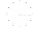
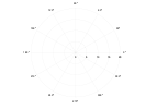
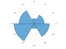
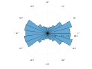
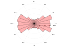
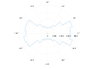
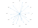
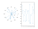
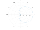
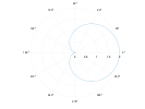
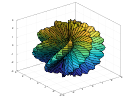
By emplacing a polar plot in the axes, the axes move to a polar mode, where we use the
From the backend point of view, these axes are an abstraction to the user. The data points in the
Aside from this conversion, these plot subcategories are analogous to line plots, scatter plots, histograms, quiver plots, and line functions.

More examples:

More examples:
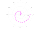
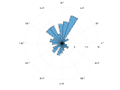
The function polarhistogram distributes the data into the number of bins provided as its second parameter.

More examples:

More examples:

More examples:
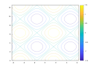
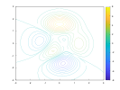
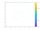
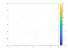
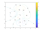
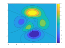
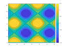
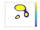
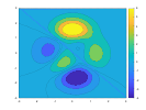
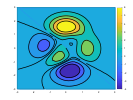
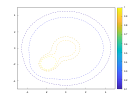
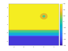
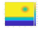
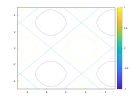
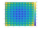
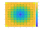
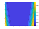
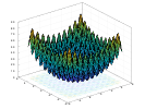
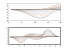
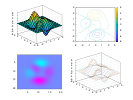
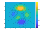
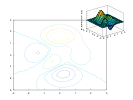
All these subcategories depend on the contours type. They also depend on lazy evaluation for generating the contour lines. When the function draw is called in the contours class, it preprocesses all contour lines for a three-dimensional function.
Although it is relatively simple to show a heatmap with the values for the contourc for calculating contour lines. This function uses an adaptation of the algorithm adopted by Matplotlib.
The algorithm creates a quad grid defined by the
Filled contours are closed polygons for pairs of contour levels. Some polygons for filled contours might be holes inside other polygons. The algorithm needs to keep track of these relationships so that we can render the polygons in their accurate order. To avoid an extra step that identifies this relationship between the polygons, the sweeping algorithm already identifies which polygons are holes for each level.
Once we find the quads with the contour line, the line is generated by interpolating the

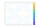
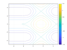
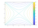
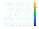
More examples:

More examples:
By default, the function fcontour will generate 9 contour lines from a lambda function. The functions contour and contourf, on the other hand, plot contour lines and filled contour lines from a grid of data points for

More examples:
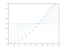
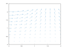
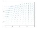
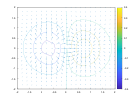
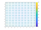
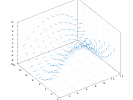
All these subcategories depend on the vectors object type. In a two-dimensional plot, for each value of
A quiver plot (or velocity plot) shows a grid of vectors whose direction and magnitude are scaled to prevent the overlap between vectors in subsequent quads.


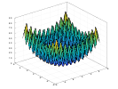
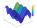
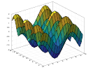
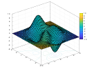
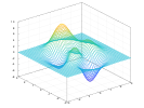
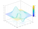
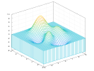
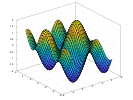
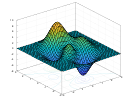
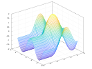
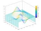
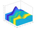
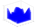
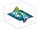
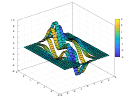
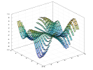
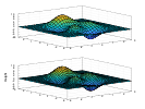
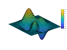
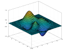
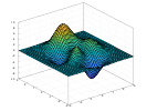
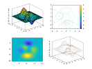
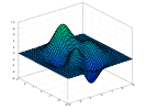
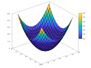
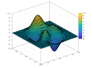
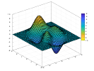
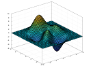
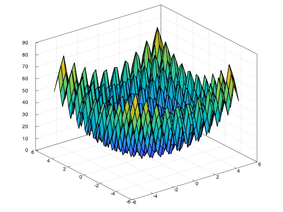
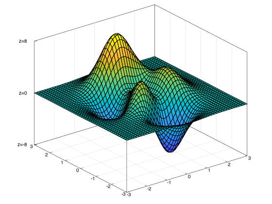
- Surface
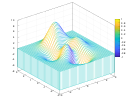
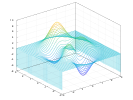
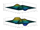
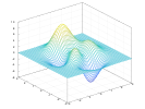
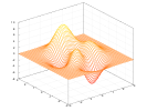
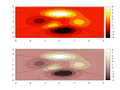
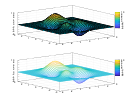
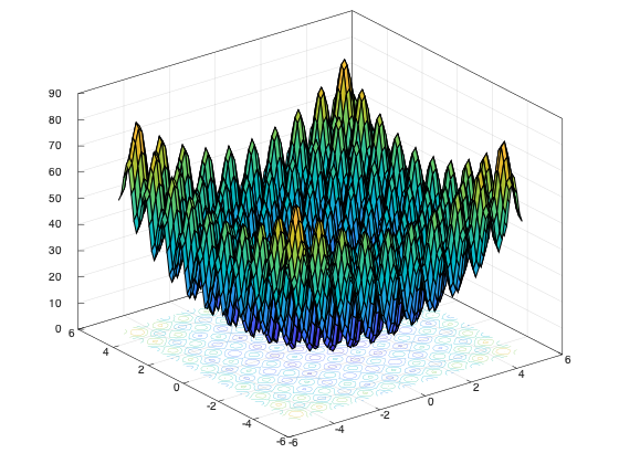
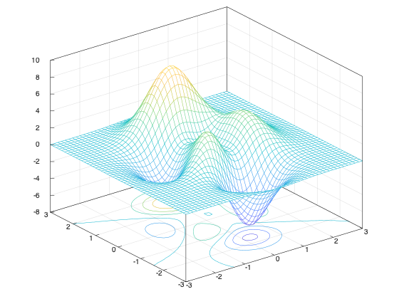
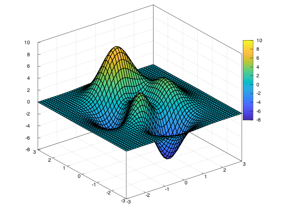
- Surface with Contour
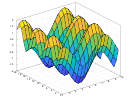
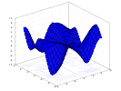
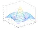
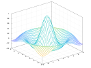
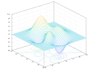
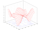
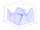
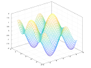
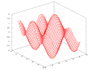
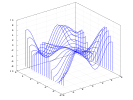
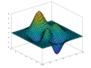
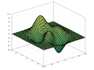
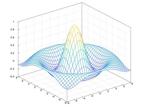
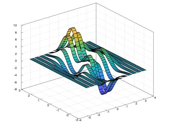
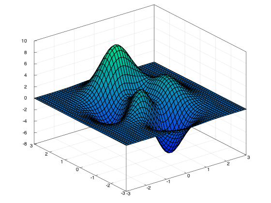
- Mesh
- Mesh with Contour
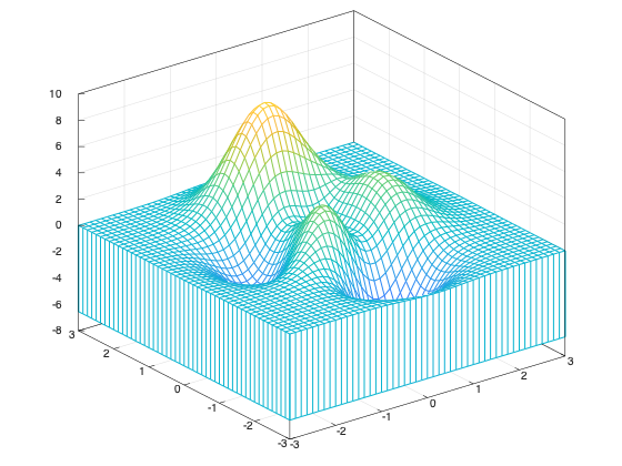
- Mesh with Curtain
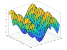
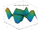
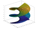
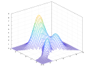
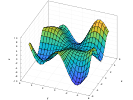
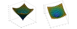
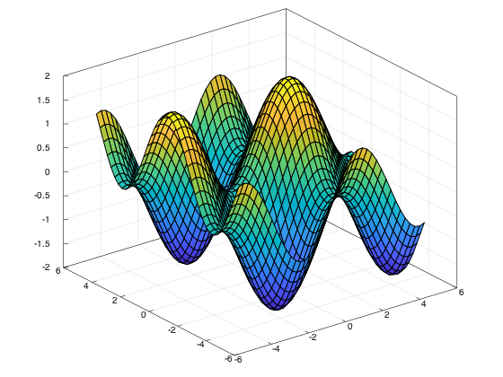
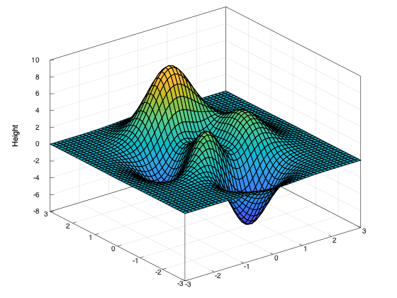
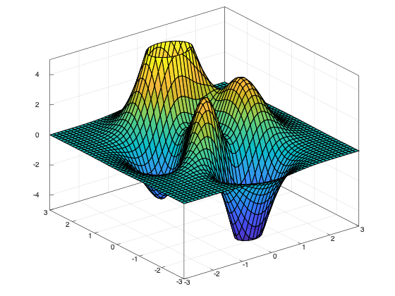
- Function Surface
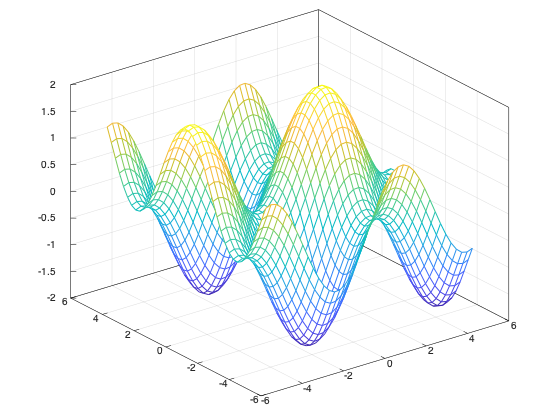
- Function Mesh
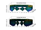
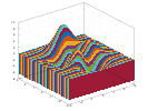
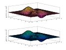
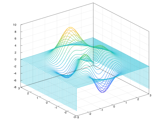
- Waterfall
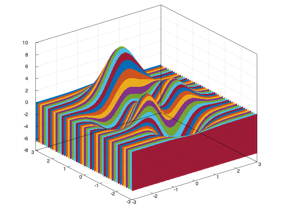
- Fence
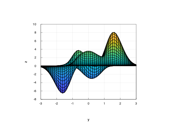
- Ribbon
More examples:
More examples:
More examples:
More examples:
More examples:
More examples:
More examples:
More examples:
More examples:
More examples:

More examples:
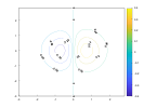
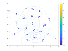
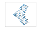
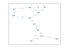
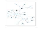
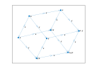
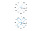
All these subcategories depend on the network class. Graphs are abstract structures that represent objects and relationships between these objects. The objects are represented as vertices and the relationships are depicted as edges.
In an abstract graph, the vertices have no specific position in space. Mathematically, a graph does not depend on its layout. However, the graph layout has a large impact on its understandability. The network class can calculate appropriate positions for graph vertices with several algorithms: Kamada Kawai algorithm, Fruchterman-Reingold algorithm, circle layout, random layout, and automatic layout.
The implementation of the Kamada Kawai and Fruchterman-Reingold algorithms depend on the NodeSoup library. The automatic layout uses the Kamada Kawai algorithm for small graphs and the Fruchterman-Reingold algorithm for larger graphs.

More examples:
More examples:
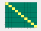
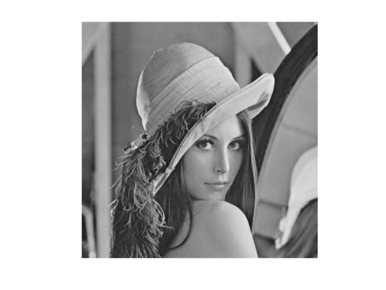
These subcategories depend on the matrix class. The matrix class can have up to four matrices. If it has only one matrix, it is represented with a colormap. If it has three matrices, they represent the red, green, and blue channels. If it has four matrices, the fourth matrix represents an alpha channel to control the transparency of each pixel.
We use the CImg library to load and save images. CImg can handle many common image formats as long as it has access to the appropriate libraries. The Matplot++ build script will look at compile-time for the following optional libraries: JPEG, TIFF, ZLIB, PNG, LAPACK, BLAS, OpenCV, X11, fftw3, OpenEXR, and Magick++. The build script will attempt to link all libraries from this list to Matplot++.
Matplot++ includes a few convenience functions to manipulate matrices with images: imread, rgb2gray, gray2rgb, imresize, and imwrite. All these functions work with lists of matrices.
More examples:

More examples:
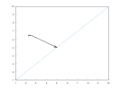
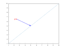
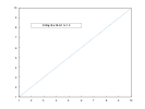
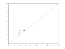
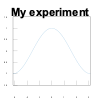
The annotations category is meant to create individual objects on the plot rather than representations of data sets. An important difference between the annotations category and other categories is that, by default, the annotations do not replace the plot that already exists in the axes object, even if the user does not call the hold function.

More examples:

More examples:

More examples:
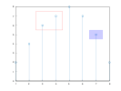
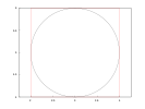
The rectangle object can have a border curvature from


![]()
More examples:
![]()

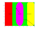
As a convenience, the colors.h header contains many functions to generate colors from strings and vice-versa.

More examples:
More examples:

More examples:

More examples:
More examples:

More examples:

More examples:

More examples:
More examples:

More examples:

More examples:

More examples:

More examples:

More examples:
More examples:

More examples:

More examples:

More examples:

More examples:

More examples:

More examples:

More examples:

More examples:

More examples:

More examples:
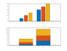
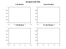
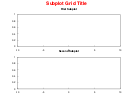
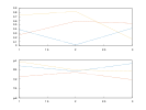
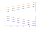
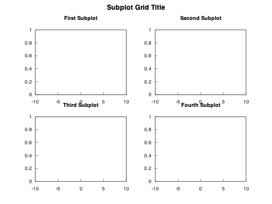
Unlike other libraries, subplots uses 0-based indices.

More examples:
Our tiling functions are convenience shortcuts for the subplot functions. If there is no room for the next tile, we automatically rearrange the axes and increase the number of subplot rows or columns to fit the next tile. Use subplots for more control over the subplots.

More examples:
More examples:
More examples:

More examples:
More examples:
More examples:

More examples:


More examples:

More examples:
The interactive plot window has a widget to save the current figure. Because this widget uses the same backend as the one used to produce the interactive image, the final image matches closely what the user sees in the window.
You can programatically save the figure in a number of formats with the save function:
save(filename);or
save(filename, fileformat);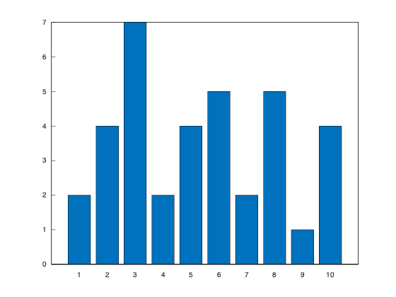
More examples:
The first option (save(filename)) infers the appropriate file format from the filename extension. In both cases (save(filename) and save(filename,fileformat)), this function temporarily changes the backend to a non-interactive backend appropriate to draw the figure. A different backend is used for each format and, depending on the format, the final image does not necessarily match what is on the interactive plot window. The reason is that some file formats purposefully do not include the same features.
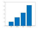
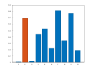
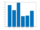
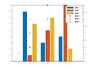
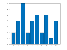
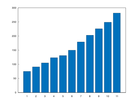
For instance, consider the bar chart generated by
vector<double> x = {29, 17, 14, 13, 12, 4, 11};
bar(x);
If we export the image with
save("barchart.svg");we get the vector graphics

Exporting the image with
save("barchart.txt");generates a representation of the image appropriate for text or markdown files, such as
       30 +-----------------------------------------------------------+
          |    *******   +       +      +       +      +       +      |
          |    *     *                                                |
       25 |-+  *     *                                              +-|
          |    *     *                                                |
          |    *     *                                                |
       20 |-+  *     *                                              +-|
          |    *     *                                                |
          |    *     ********                                         |
       15 |-+  *     **     *                                       +-|
          |    *     **     * *******                                 |
          |    *     **     * *     ******** *******                  |
          |    *     **     * *     **     * *     *        *******   |
       10 |-+  *     **     * *     **     * *     *        *     * +-|
          |    *     **     * *     **     * *     *        *     *   |
          |    *     **     * *     **     * *     *        *     *   |
        5 |-+  *     **     * *     **     * *     ******** *     * +-|
          |    *     **     * *     **     * *     **     * *     *   |
          |    *  +  **  +  * *  +  **  +  * *  +  **  +  * *  +  *   |
        0 +-----------------------------------------------------------+
                  1      2       3      4       5      6       7
As the last example, saving an image with
save("barchart.tex");would save the image in a format appropriate to embed in latex documents, such as

This exports the image in a format in which the labels are replaced by latex text so that the plot fits the rest of the document.
Like in Matplotlib, we support two coding styles: Free-standing functions and an Object-oriented interface.
-
Freestanding functions:
- We call functions to create plots on the current axes
- The global current
axesobject is the currentaxesobject in the current figure in the global figure registry - For instance, one can use
plot(y);to create a line plot on the current axes (or create a newaxesobject if needed). - Also, one can use
plot(ax,y);to create a line plot on theaxesobjectax. - This is less verbose for small projects and quick tests.
- The library looks for existing axes to create the plot.
-
Object-oriented interface:
- We explicitly create figures and call methods on them
- For instance, one can use
ax->plot(y);to plot on theaxesobjectax - We can create the same line plot on the current axes by
auto ax = gca(); ax->plot(y); - This is less verbose and provides better control in large projects where we need to pass these objects around
- The user manages axes handles containing plots.
Assuming the user is explicitly managing the axes to create plots in another function, a more complete example of these styles could be
// Free-standing functions
auto ax = gca();
plot(ax, x, y)->color("red").line_width(2);
my_function(ax);
and
// Object-oriented interface
auto ax = gca();
ax->plot(x, y)->color("red").line_width(2);
my_function(ax);
Both examples would generate the same plot. All free-standing functions are templated functions that use meta-programming to call the main function on the current axes object. If the first parameter is not an axes_handle, it will get an axes_handle from the figure registry with gca (Section Figures and Axes) and forward all parameters to the function in this axes object. If the first parameter is an axes_handle, the template function will forward all parameters, but the first one, to this axes object. This use of templates for the free-standing functions keeps both coding styles maintainable by the developers.
Note that, because the example needs the axes object for the function my_function, we also need to get a reference to the axes object with the free-standing functions. In that case, the free-standing functions are not less verbose than the object-oriented interface.
To adhere to free-standing functions, we could create two versions of my_function: one that receives an axes_handle, and a second version that would get an axes_handle from the figure registry and call the first version. If my_function is going to be exposed to other users as a library, this could be a convenience to these users. However, notice that this is only moving the verbosity from the main function to my_function. In fact, this is how the free-standing functions in Matplot++ work.
There are also two modes for figures: reactive (or interactive) mode and quiet mode. Figures in reactive mode are updated whenever any of their child objects change. This happens through the touch function, that gets called on any child object when it changes its appearance. This creates an interactive mode in which figures are updated as soon as we adjust their properties. If we combine interactive figures with free-standing functions, we have a "Matlab-like style" for plots. This is a coding pattern where the figure registry works as a stream for plots.
The problem with this coding style is that the user might unnecessarily create useless intermediary plots.
Figures in quiet mode are updated by calling the functions draw() or show() (Section Figures and Axes). Unless these functions are called, nothing changes in the figure. The combination of the object-oriented coding style and quiet mode is the "OO-Matplotlib-like style" for plots. This is a coding style in which the user explicitly decides when the plot is shown or updated. This is beneficial to applications that cannot waste computational resources on intermediary figures that might not be valuable to the application.
We generally use free-standing functions with reactive mode and the object-oriented interface with quiet mode. By default, new figures are in reactive mode, unless it is using an non-interactive backend. One can turn this reactive mode on and off with:
ion()orioff()free-standing functionsreactive(bool)orquiet(bool)function on thefigureobjectfigure(true)orfigure(false)when explicitly creating a new figure
A more complete example of the reactive mode would be:
// Reactive mode
auto f = gcf(false);
auto ax = f->gca();
auto p = ax->plot(ax, x, y);   // draws once
p->color("red").line_width(2); // draws twice more
wait();                        // pause console
For convenience, the examples in Section Plot Categories use the reactive mode. The wait function pauses the console until the user interacts with the plot window. If the backend is based on process pipes, because these are unidirectional, closing the window is not enough to resume. The user needs to use the console to unblock execution. A similar example is quiet mode would be
// Quiet mode
auto f = gcf(true);
auto ax = f->gca();
auto p = ax->plot(x,y);        // does not draw
p->color("red").line_width(2); // does not draw
f->show();                     // draw only once and pause console
In this example, the figure is only updated once. The user could replace the show function with the draw function, but the window would close as soon as execution completes. It is important to use wait() and show() with caution. These functions are meant for some particular executables so that an interactive plot does not close before the user can see it. It is probably unreasonable to call these functions inside a library because the user would have to manually interfere with the execution to continue.
To support a more compact syntax, the library allows method chaining on plot objects. For instance, we can create a simple line plot and modify its appearance by
// Using the line handle
auto p = plot(x,y,"--gs");
p->line_width(2);
p->marker_size(10);
p->marker_color("b");
p->marker_face_color({.5,.5,.5});
or
// Method chaining
plot(x,y,"--gs")->line_width(2).marker_size(10).marker_color("b").marker_face_color({.5,.5,.5});
The first code snippet works because plot returns a line_handle to the object in the axes. We can use this line handle to modify the line plot. Whenever we modify a property, the setter function calls touch, which will draw the figure again if it is in reactive mode. The second option works because setters return a reference to *this rather than void.
The plotting functions work on any range of elements convertible to double. For instance, we can create a line plot from a set of elements by
set<int> y = {6,3,8,2,5};
plot(y);
Any object that has the functions begin and end are considered iterable ranges. Most axes object subclasses use vector<double> or vector<vector<double>> to store their data. For convenience, the common.h header file includes the aliases vector_1d and vector_2d to these data types.
These conversions also work on ranges of ranges:
vector<set<int>> Y = {{6,3,8,2,5},{6,3,5,8,2}};
plot(Y);
Unfortunately, because of how templated functions work, one exception is initializer lists. Initializer lists only work for functions that are explicitly defined for them.
The headers common.h and colors.h include a number of utilities we use in our examples. These include naive functions to generate and manipulate vectors and strings; handle RGBA color arrays; convert points to and from polar coordinates; read files to strings; write strings to files; calculate gradients; read, write, and manipulate images; and generate vectors with random numbers. Although some of these functions might be helpful, most functions only operate on vector<double> and they are not intended to be a library of utilities. The sole purpose of these algorithms is to simplify the examples.
If you are interested in understanding how the library works, you can read the details in the complete article. It describes the relationship between its main objects, the backend interface, how to create new plot categories, limitations, and compares this library with similar alternatives.
Check if you have Cmake 3.14+ installed:
cmake -versionDownload the whole project and add the subdirectory to your Cmake project:
add_subdirectory(matplotplusplus)When creating your executable, link the library to the targets you want:
add_executable(my_target main.cpp)
target_link_libraries(my_target PUBLIC matplot)
Add this header to your source files:
#include <matplot/matplot.h>Check if you have Cmake 3.14+ installed:
cmake -versionInstall CPM.cmake and then:
CPMAddPackage(
    NAME matplotplusplus
    GITHUB_REPOSITORY alandefreitas/matplotplusplus
)
# ...
target_link_libraries(my_target PUBLIC matplot)
Then add this header to your source files:
#include <matplot/matplot.h>If you're not using Cmake, your project needs to include the headers and compile all source files in the source directory. You also need to link with the dependencies described in source/matplot/FindDependencies.cmake.
Then add this header to your source files:
#include <matplot/matplot.h>This project requires C++17. You can see other dependencies in FindDependencies.cmake. CMake will try to solve everything for you.
- Required
- olvb/nodesoup (CMake will download it for you)
- dtschump/CImg (CMake will download it for you)
- Gnuplot (for the Gnuplot backend only)
- Optional (for images)
- JPEG
- TIFF
- ZLIB
- PNG
- LAPACK
- BLAS
- FFTW
- OpenCV
- OPENEXR
- MAGICK
There's an extra target matplot_opengl that exemplifies how an OpenGL backend could be implemented. It's not a complete backend. If you want to test it, only then there are some extra dependencies.
- Dependencies for the OpenGL backend
- OpenGL
- GLAD
- GLFW3
Coming up with new backends is a continuous process. See the complete article for a description of the backend interface, a description of the current default backend (Gnuplot pipe), and what's involved in possible new backends. See the directory source/matplot/backend for some examples. Also, have a look at this example test/backends/main.cpp.
There are many ways in which you can contribute to this library:
- Testing the library in new environments
- Contributing with interesting examples
- Designing new backends see 1, 2, 3
- Finding problems in this documentation
- Writing algorithms for new plot categories
- Finding bugs in general
- Whatever idea seems interesting to you
-
Abadi M, Barham P, Chen J, Chen Z, Davis A, Dean J, Devin M, Ghemawat S, Irving G,Isard M,et al.(2016). "Tensorflow: A system for large-scale machine learning." In 12th USENIX symposium on operating systems design and implementation (OSDI 16), pp.265-283.
-
Angerson E, Bai Z, Dongarra J, Greenbaum A, McKenney A, Du Croz J, Hammarling S,Demmel J, Bischof C, Sorensen D (1990). "LAPACK: A portable linear algebra library for high-performance computers." In Supercomputing'90: Proceedings of the 1990 ACM/IEEE Conference on Supercomputing, pp. 2-11. IEEE.
-
Antcheva I, Ballintijn M, Bellenot B, Biskup M, Brun R, Buncic N, Canal P, Casadei D, CouetO, Fine V, et al.(2011). "ROOT-A C++ framework for petabyte data storage, statistical analysis and visualization."Computer Physics Communications,182(6), 1384-1385.
-
Baratov R (2019). Hunter. URL: https://hunter.readthedocs.io.
-
Barrett P, Hunter J, Miller JT, Hsu JC, Greenfield P (2005). "matplotlib-A Portable Python Plotting Package." In Astronomical data analysis software and systems XIV, volume 347,p. 91.
-
Bezanson J, Edelman A, Karpinski S, Shah VB (2017). "Julia: A fresh approach to numerical computing. "SIAM review,59(1), 65-98.
-
CEGUI Team (2020). CEGUI. URL: http://cegui.org.uk.
-
Cornut O (2020). Dear ImGui: Bloat-free Immediate Mode Graphical User Interface for C++ with minimal dependencies. URL: https://github.com/ocornut/imgui.
-
de Guzman J (2020). Elements. URL: http://cycfi.github.io/elements/.
-
Eichhammer E (2020). QCustomPlot. URL: https://www.qcustomplot.com.
-
Evers B (2019). Matplotlib-cpp. URL: https://github.com/lava/matplotlib-cpp.
-
Freitas A (2020). Pareto Front Library. URL: https://github.com/alandefreitas/pareto-front.
-
Frigo M, Johnson SG (1998). "FFTW: An adaptive software architecture for the FFT." In Proceedings of the 1998 IEEE International Conference on Acoustics, Speech and Signal Processing, ICASSP'98 (Cat. No. 98CH36181), volume 3, pp. 1381-1384. IEEE.
-
Fruchterman TM, Reingold EM (1991). "Graph drawing by force-directed placement. "Software: Practice and experience, 21(11), 1129-1164.
-
GNU Project (2020). GNU Octave: Introduction to Plotting. URL: https://octave.org/doc/v4.2.2/Introduction-to-Plotting.html.
-
Guy Eric Schalnat Andreas Dilger GRP (2020). Libpng. URL: https://sourceforge.net/p/libpng/.
-
Hao J (2020). Nana. URL: http://nanapro.org/.
-
Hunter JD (2007). "Matplotlib: A 2D graphics environment. "Computing in Science & Engineering, 9(3), 90-95. doi:10.1109/MCSE.2007.55.
-
Idea4good (2020). GuiLite. URL: https://github.com/idea4good/GuiLite.
-
ImageMagick Studio LLC (2020). Magick++. URL: https://imagemagick.org/Magick++/.
-
Independent JPEG Group (2020). Libjpeg. URL: http://libjpeg.sourceforge.net.
-
Intel Corporation, Willow Garage I (2020). Open Source Computer Vision Library (OpenCV). URL: https://opencv.org/.
-
Jakob W (2017). PyBind11. URL: https://pybind11.readthedocs.io/en/stable/.
-
Kagstrom B LP, C VL (2020). Basic Linear Algebra Subprograms (BLAS). URL: http://www.netlib.org/blas/.
-
Kainz F, Bogart R, Hess D (2003). "The OpenEXR image file format."SIGGRAPH TechnicalSketches.
-
Kamada T, Kawai S,et al.(1989). "An algorithm for drawing general undirected graphs."Information processing letters,31(1), 7-15.
-
Loup Gailly J, Adler M (2020). Zlib. URL: https://github.com/madler/zlib.
-
Martin K, Hoffman B (2010). Mastering CMake: a cross-platform build system. Kitware.
-
McKinney W,et al.(2011). "Pandas: a foundational Python library for data analysis and statistics. "Python for High Performance and Scientific Computing, 14(9).
-
Conan.io (2020). Conan. URL: https://conan.io.
-
Melchior L (2020). CPM.cmake. URL: https://github.com/TheLartians/CPM.cmake.
-
Murray Cumming DE (2020). Gtkmm. URL: https://www.gtkmm.org/.
-
Natural Earth (2018). "Natural earth. Free vector and raster map data." URL: http://www.naturalearthdata.com/downloads/.
-
NetworkX developers (2020). NetworkX. URL: https://networkx.github.io.
-
OLVB (2020). Node Soup. URL: https://github.com/olvb/nodesoup.
-
Pezent E (2020). ImPlot. URL: https://github.com/epezent/implot.
-
Sam Leffler SG (2020). Libtiff. URL: https://gitlab.com/libtiff/libtiff.
-
Schaling B (2011). The boost C++ libraries. Boris Schaling.
-
Spitzak B, et al.(2004). "Fast Light Toolkit (FLTK)." FTLK: Fast light toolkit. Available: http://www.fltk.org/
-
Stahlke D (2020). Gnuplot-Iostream. URL: http://stahlke.org/dan/gnuplot-iostream/.
-
Storer J (2020). JUCE. URL: https://juce.com.
-
Terra Informatica Software, Inc (2020). Sciter. URL: https://sciter.com.
-
The FLTK Team (2020). FLTK. URL: https://www.fltk.org.
-
The MathWorks, Inc (2020). MatlabGraphics. URL: https://www.mathworks.com/help/matlab/graphics.html.
-
The Qt Company (2020). Qt. URL: https://www.qt.io.
-
Tschumperle D (2020). CImg. URL: http://cimg.eu.
-
van der Zijp J (2020). Fox toolkit. URL: http://fox-toolkit.org.
-
Vasilev V, Canal P, Naumann A, Russo P (2012). "Cling-the new interactive interpreter for root 6." In Journal of Physics: Conference Series, volume 396, p. 052071.
-
Walt Svd, Colbert SC, Varoquaux G (2011). "The NumPy array: a structure for efficient numerical computation." Computing in science & engineering,13(2), 22-30.
-
Wei V (2020). MiniGUI. URL: http://www.minigui.com.
-
Williams T, Kelley C, Bersch C, Broker HB, Campbell J, Cunningham R, Denholm D, Elber G, Fearick R, Grammes C,et al.(2017). "gnuplot 5.2."
-
wxWidgets (2020). WxWidgets. URL: https://wxwidgets.org.
-
XOrg Foundation (2020). X11. URL: https://www.x.org/.
-
Zaitsev S (2020). Webview. URL: https://github.com/zserge/webview.
-
Zakai A (2011). "Emscripten: an LLVM-to-JavaScript compiler." In Proceedings of the ACM international conference companion on Object oriented programming systems languages and applications companion, pp. 301-312.