shukkkur / Classify-Song-Genres-from-Audio-Data

Python ML Methods to classify songs into genres.

Classify Song Genres from Audio Data
Rock or rap?

---

1. Preparing our dataset

Over the past few years, streaming services with huge catalogs have become the primary means through which most people listen to their favorite music. For this reason, streaming services have looked into means of categorizing music to allow for personalized recommendations.

Let's load the metadata about our tracks alongside the track metrics compiled by The Echo Nest.

import pandas as pd

tracks = pd.read_csv('datasets/fma-rock-vs-hiphop.csv')
echonest_metrics = pd.read_json('datasets/echonest-metrics.json', precise_float=True)

# Merge the relevant columns of tracks and echonest_metrics
echo_tracks = pd.merge(echonest_metrics, tracks[['track_id' , 'genre_top']], how='inner', on='track_id')

# Inspect the resultant dataframe
echo_tracks.info()

Int64Index: 4802 entries, 0 to 4801
Data columns (total 10 columns):
acousticness	4802 non-null float64
danceability	4802 non-null float64
energy	4802 non-null float64
instrumentalness	4802 non-null float64
liveness	4802 non-null float64
speechiness	4802 non-null float64
tempo	4802 non-null float64
track_id	4802 non-null int64
valence	4802 non-null float64
genre_top	4802 non-null object
dtypes: float64(8), int64(1), object(1)
memory usage: 412.7+ KB

2. Pairwise relationships between continuous variables

We want to avoid using variables that have strong correlations with each other -- hence avoiding feature redundancy
To get a sense of whether there are any strongly correlated features in our data, we will use built-in functions in the pandas package .corr().

corr_metrics = echo_tracks.corr()
corr_metrics.style.background_gradient()

3. Normalizing the feature data

Since we didn't find any particular strong correlations between our features, we can instead use a common approach to reduce the number of features called principal component analysis (PCA)
To avoid bias, I first normalize the data using sklearn built-in StandardScaler method

from sklearn.preprocessing import StandardScaler

features = echo_tracks.drop(['track_id', 'genre_top'], axis=1)
labels = echo_tracks.genre_top

scaler = StandardScaler()
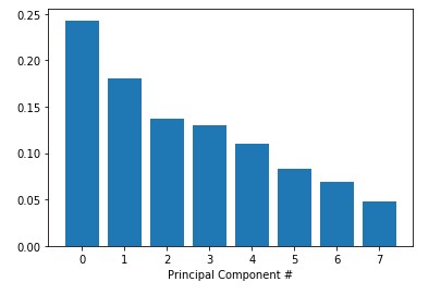
scaled_train_features = scaler.fit_transform(features)

4. Principal Component Analysis on our scaled data

Now PCA is ready to determine by how much we can reduce the dimensionality of our data. We can use scree-plots and cumulative explained ratio plots to find the number of components to use in further analyses.
When using scree plots, an 'elbow' (a steep drop from one data point to the next) in the plot is typically used to decide on an appropriate cutoff.

from sklearn.decomposition import PCA

pca = PCA()
pca.fit(scaled_train_features)

exp_variance = pca.explained_variance_ratio_

fig, ax = plt.subplots()
ax.bar(range(pca.n_components_), exp_variance)

Unfortunately, there does not appear to be a clear elbow in this scree plot, which means it is not straightforward to find the number of intrinsic dimensions using this method.

5. Further visualization of PCA

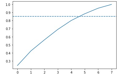
Let's nownlook at the cumulative explained variance plot to determine how many features are required to explain, say, about 85% of the variance

cum_exp_variance = np.cumsum(exp_variance)

fig, ax = plt.subplots()
ax.plot(cum_exp_variance)
ax.axhline(y=0.85, linestyle='--')

# choose the n_components where about 85% of our variance can be explained
n_components = 6

pca = PCA(n_components, random_state=10)
pca.fit(scaled_train_features)
pca_projection = pca.transform(scaled_train_features)

6. Train a decision tree to classify genre

Now we can use the lower dimensional PCA projection of the data to classify songs into genres. we will be using a simple algorithm known as a decision tree.

from sklearn.model_selection import train_test_split
from sklearn.tree import DecisionTreeClassifier

train_features, test_features, train_labels, test_labels = train_test_split(pca_projection, labels, random_state=10)

tree = DecisionTreeClassifier(random_state=10)
tree.fit(train_features, train_labels)

pred_labels_tree = tree.predict(test_features)

7. Compare our decision tree to a logistic regression

There's always the possibility of other models that will perform even better! Sometimes simplest is best, and so we will start by applying logistic regression.

from sklearn.linear_model import LogisticRegression
from sklearn.metrics import classification_report

logreg = LogisticRegression(random_state=10)
logreg.fit(train_features, train_labels)
pred_labels_logit = logreg.predict(test_features)

class_rep_tree = classification_report(test_labels, pred_labels_tree)
class_rep_log = classification_report(test_labels, pred_labels_logit)

print("Decision Tree: \n", class_rep_tree)
print("Logistic Regression: \n", class_rep_log)

Decision Tree:
precision	recall	f1-score	support
Hip-Hop	0.66	0.66	0.66	229
Rock	0.92	0.92	0.92	972
avg / total	0.87	0.87	0.87	1201

Logistic Regression:
precision	recall	f1-score	support
Hip-Hop	0.75	0.57	0.65	229
Rock	0.90	0.95	0.93	972
avg / total	0.87	0.88	0.87	1201

8. Using cross-validation to evaluate our models

To get a good sense of how well our models are actually performing, we can apply what's called cross-validation (CV).

from sklearn.model_selection import KFold, cross_val_score

kf = KFold(n_splits=10)

tree = DecisionTreeClassifier(random_state=10)
logreg = LogisticRegression(random_state=10)

tree_score = cross_val_score(tree,pca_projection, labels, cv=kf)
logit_score = cross_val_score(logreg,pca_projection, labels, cv=kf)

print("Decision Tree:", tree_score)
>>> Decision Tree: [0.6978022  0.6978022  0.69230769 0.78571429 0.71978022 0.67032967 0.75824176 0.76923077 0.75274725 0.6978022 ]
print("Logistic Regression:", logit_score)
>>> Logistic Regression: [0.79120879 0.76373626 0.78571429 0.78571429 0.78571429 0.78021978 0.75274725 0.76923077 0.81868132 0.71978022]

Success!