Data Analysis Pipeline

The purpose of the pipeline in this repository is to provide analysis tools that can eliminate and reduce boring and repetitive tasks in data analysis.

Pipeline

"my_pipeline" directory provides analysis tools for load/save files, data cleaning/feature engineering and modelling. The pipeline can be used for future data analysis and reduce coding tasks.

Analysis Codes

In this repository, there are two codes to analyse data:

TitanicSurvivorPrediction.py
UberDemandPrediction.py

These analysis codes were developed based on the insights obtained from Exploratory Data Analysis (EDA) on a jupyter notebook (see links below). Titanic survival prediction is a binary classification task and Uber demand forecasting is time-series forecasting. These are different types of tasks, but some basic analysis can be done with common analysis tools.

Links

(Titanic survivor prediction)
Jupyter Notebook
https://github.com/shotashirai/Data-Analysis-Pipeline/blob/main/EDA_Jupyter_Notebook/TitanicSurvivalPrediction_EDA_Model.ipynb
Original Repository
https://github.com/shotashirai/Titanic-Survival-Prediction

(Uber Demand Forecasting)
Jupyter Notebook
https://github.com/shotashirai/Data-Analysis-Pipeline/blob/main/EDA_Jupyter_Notebook/Uber-Demand-Forecasting_EDA_Model.ipynb
Original Repository
https://github.com/shotashirai/Uber-Demand-Forecasting-NYC

Optimization of the Code - UberDemandForecasting

(Updated: 31 Oct 2021)

Review of the code

cProfile, line_profiler and memory_profiler were used for the initial review of the codes. The profile (.stats) obtained by python -m cProfile -o file_name.stats my_script.py can be visualized using snakeviz file_name.stats

These tools found that:

data_profile() took ~37s to obtain the information of the DataFrame, especially duplication check is the most time-consuming.
datetime_format() is also time-consuming (~10s)
Multiple Pandas DataFrames need memory, which may affect the performance of the data_profile().
Modelling section is very time-consuming (10min to get results), especially feature selection using BorutaPy.

(ref)
line_profiler: https://github.com/rkern/line_profiler
memroy_profiler: https://github.com/pythonprofilers/memory_profiler

Optimization methods

The major approaches to optimize the performance are:

Replace custom-made functions with built-in functions where possible.
Use memory-efficient data types based on EDA.
Not create/copy unnecessary DataFrames.
Restructure the code.

*1 Multiprocessing on CPU is already used in some models.
*2 Multiprocessing on GPU is not considered at this stage.

Optimization

Data types in DataFrames

The data types automatically selected by Pandas are usually int64, float64 or object which needs more memory. To reduce the memory usage, other memory-efficient data types (int16, int8, float32, category) were selected based on the insights from EDA. The result of the optimization of the data types is shown in the table below. Memory usage for DataFrames of Uber data and weather data were drastically improved after changing the data types.

	Before optimization	After optimization
Uber data	4.4GB	122.5MB
Weather data	564.6KB	82.4KB
Location ref	37.8KB	1.6KB
df_model	8.2MB	7.9MB

* df.info(memory_usage='deep') is used for memory usage measurements.

BorutaPy

Boruta is a strong feature selection algorithm designed as a wrapper around a Random Forest classification algorithm. However, it is slow. In this code, the feature selection by Boruta is the main bottleneck for efficient computation. Boruta is normally implemented with Random Forest classification, but other models can be used and result in better performance. (ref: scikit-learn-contrib/boruta_py#80)

To compare the performance, three regressor models (Random Forest, XGBoost, lightGBM) were tested. The table below shows the elapsed time to select features and the accuracy of the prediction (MAPE: Mean Absolute Percentage Error). All models show very similar accuracy values (1.6 +/- 0.1%), but lightGBM shows a significant improvemnt of the performance for efficient computation. So, an optimized version of the code, lightGBM is used for feature selection with BorutaPy.

Model	Elapsed time	Accuracy (MAPE)
Random Forest Regressor	~176s	1.7%
XGBoost	~170s	1.5%
lightGBM	~26s	1.63%

Restructuring code

Import data

This section loads data and prepares for further analysis in later sections.

load_file() was removed due to less flexibility to load files.
A code to load data from .csv files was directly written on the main code to select data attributes and proper data types.
Weather data is loaded using glob module that allows getting a list of files in a directory. Data types are selected after generating a weather DataFrame (df_weather).
Weather data with a period (2015-01-01 - 2015-06-30) is extracted in the loading section, leading to memory usage reduction.

To create/format DataFrame is done in this section and the section of 'Preprocessing for analysis' is not needed anymore.

Preprocessing

The "Preprocessing" section get hourly statistics of Uber rides and concatenates the Uber data and the weather data.

A single DataFrame (df_uber_hourly) obtained from the original Uber DataFrame contains all required variables (e.g., rides for each borough).
df_model used for modelling are created from df_uber_hourly and df_weather.

While the old code generated multiple DataFrames, the optimized code minimizes creating DataFrames which helps to reduce memory usage.

Model Deployment

This section builds and trains XGBoost model and implement time-series forecasting using the trained model.

prediction_XGBoost() is removed because it is complicated and is likely to cause low readability and low maintainability.
TimeSeries_XGBoost() was created. This function simply trains and return predicted values for time-series data. XGBoost (regressor) is used as a model.
Model building and feature selection have been done outside of the model deployment function. This way makes it easy to read the code and tune parameters.
As mentioned in the section above (BorutaPy), lightGBM is used for feature selection with BorutaPy.

Function: data_profile()

This function returns the profile of a DataFrame. To improve the performance,

replace an original method with a built-in function
reduce DataFrames created and use a single DataFrame to store the information

Function: gen_lagdata()

This function is used for generating lag features. In the optimized version,

removed df.copy()
reduce variables created
use df.shift(lag) to generate lag feature and df.drop() to remove NaN values.

These changes made the function simple and short.

Results of Optimization

Time Efficiency

time python UberDemandPrediction.py measures the elapsed time to run the entire code. Elapsed time for each code section was measured with the time() module. As shown in the table below, the performance of the code is significantly improved (reduce computation time by ~60%) after optimization.

	Before optimization	After optimization
Elapsed time (real)	14m36s	4m21s
(Section)
Import data - preprocessing	19.7s	11.3s
Data Profile	37.2s	2.1s
Preprocessing	9.4s	8.6s
Feature Engineering	0.5s	0.2s
Model Deployment	513s	186s

Memory usage

Memory usage of the major DataFrames

Memory usage for major DataFrames is also drastically improved by using proper data types as shown below.

	Before optimization	After optimization
Uber data	4.4 GB	122.5MB
Weather data	564.6KB	82.4KB
Location ref	37.8KB	1.6KB
df_model	8.2MB	7.9MB

* df.info(memory_usage='deep') is used for memory usage measurements.

Memory usage in time

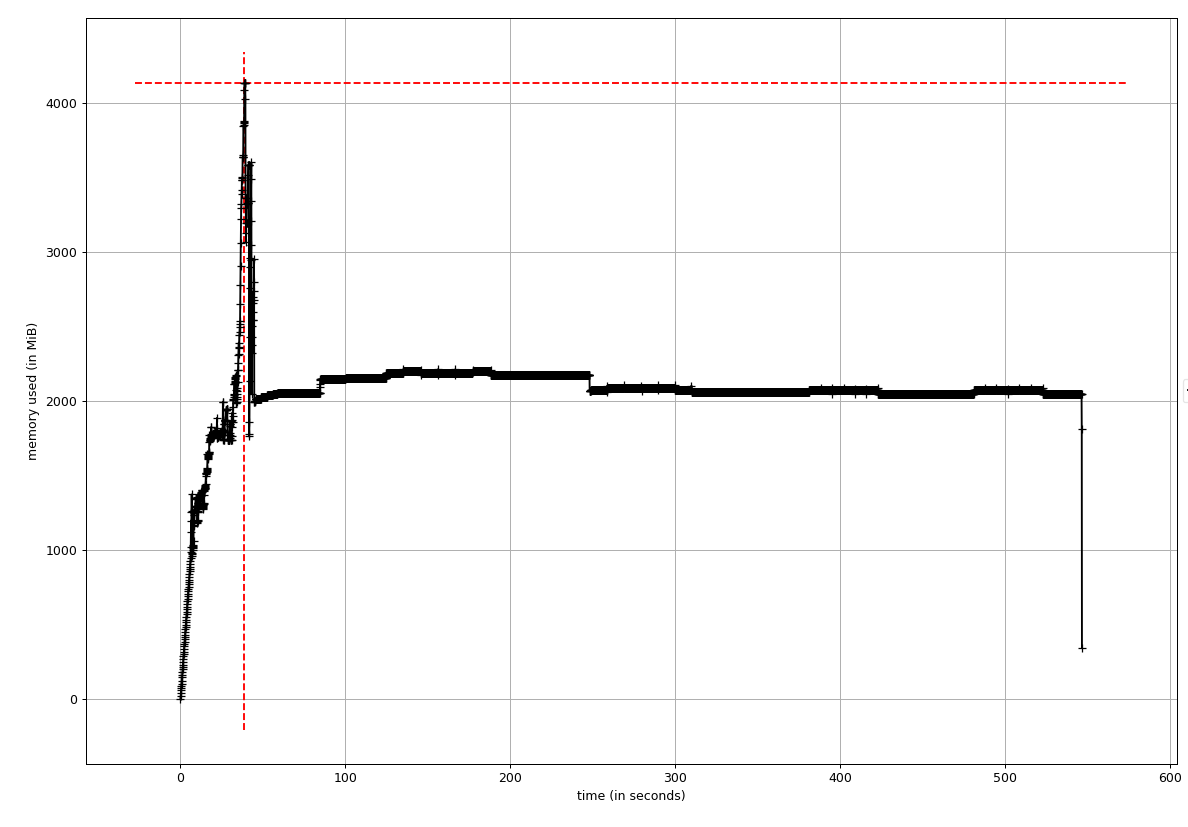
mprof run -M python UberDemandPrediction.py measures the memory usage over time and mprof plot provides a trace of the memory usage.

--- Before Optimization ---

Peak memory consumption was ~4GB
The memory usage stayed at ~2GB after the peak

--- After Optimization ---

Peak memory consumption was ~2GB
The memory usage stayed at below 500MB after the peak

Readability of the code

After optimization, the readability of the code is enhanced.

Note

test directory contains the test code used for optimization.
archived directory contains the old code.
code_profile directory stores profile obtained by cProfile. These can be visualized using snakeviz UberProfile.stats

Review of the code - Titanic Survivor Prediction

The code for titanic survivor prediction has a small bug (feature selection was implemented for each model). To fix the bugs, cls_model_deployer() was modified. The elapsed time before and after fixing the bugs are shown in the table below. As can be seen, the performance of the code is slightly improved.

	Before fixing bugs	After fixing bugs
Elapsed time (real)	44s	31s

shotashirai / Data-Analysis-Pipeline