neural-g

An R package for implementing neural-g, a neural network-based approach for g-modeling, or mixing density estimation in a latent variable model.

Abstract

Neural-g is a flexible neural network-based approach for estimating the mixing density in a latent variable model. Neural-g is capable of estimating a variety of latent densities, including atomic, smooth, flat, piecewise constant, and heavy-tailed densities. Neural-g works well under default hyperparameters that do not require additional tuning.

Installation

To run the neural-g smoothly, there are several prerequisites that need to be installed before using the R package. The main functions neural_g and neural_g2 are written in Python, namely the Pytorch library. We strongly recommend using CUDA (GPU-Based tool) to train neural-g, which offers magnitudes of speedup over using CPU.

Python 3.7 or above
Pytroch 1.11.0 or above
NAVID CUDA 10.2 or above

In R, we also need reticulate package to run Python in R and devtools to install R package from github.

install.package("reticulate")
install.package("devtools")

Now, use the following code to install neuralG package.

library(devtools)
install_github(repo = "shijiew97/neuralG")
library(neuralG)

Main function

There are two main functions in the neuralG package, which are detailed below.

neural_g gives the neural-g estimator for a univariate mixture model. Currently neural_g supports the following mixture models: Gaussian-location, Poisson-mixture, Lognormal-location, Gumbel-location, Gaussian-scale, Binomial-prob.
neural_g2 gives the bivariate neural-g estimator for a bivariate mixture model. Currently neural_g2 supports Gaussian location-scale mixture model.

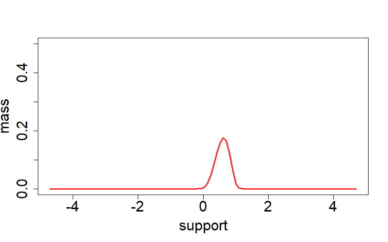
Example (1) : Lognormal-location (Beta) mixture.

As a simple example of neuralG pacakge, we consider a Lognorm-location mixture: $\mathbf{Y} \mid \theta \sim \text{Log-normal}(\theta, 1/5) \text{ and } \theta \sim \text{Beta}(3,2)$ where latent distribution follows $\text{Beta}(3,2)$ have a support of $[0,1]$ and $n=2,000$.

Seed <- 128783;set.seed(Seed);dist <- "LogGaussian";param <- 0.2
n <- 2000;L <- 5;num_it <- 4000;n_grid <- 100
theta <- rbeta(n, 3, 2);Y = rlnorm(n, theta, param)
net_g <- neural_g(Y=Y, param=param, dist=dist, n=n, num_it=num_it, n_grid=n_grid)
plot(net_g$support, net_g$prob, col=rgb(1,0,0,0.8), type='l',
     xlab='support', ylab='mass', lwd=3, ylim=c(0, 0.5), cex.axis=1.85, cex.lab=1.85)

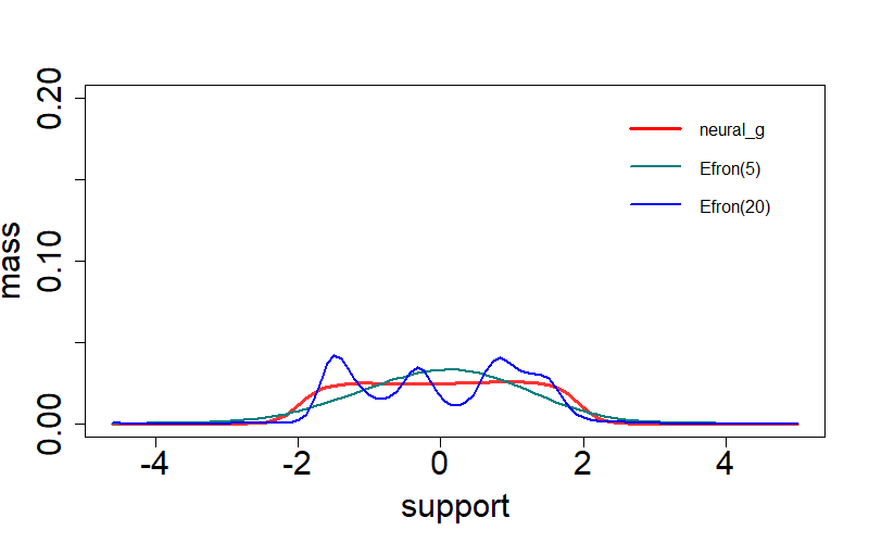
Example (2) : Gaussian-location (Uniform) mixture.

Here we also consider Efron's $\widehat{g}$ estimator in a Gaussian-location (Uniform) mixutre: $\mathbf{Y} \mid \theta \sim \mathcal{N}(\theta,1) \text{ and } \theta \sim \mathcal{U}\text{nif}(-2,2)$ where $n=2,000$.

Seed <- 128783;set.seed(Seed);dist <- "Gaussian";param <- 1.0
n <- 4000;L <- 5;num_it <- 4000;n_grid <- 100
theta <- runif(n, -2, 2);Y = theta + rnorm(n, 0, param)
net_g <- neural_g(Y=Y, param=param, dist=dist, n=n, num_it=num_it, n_grid=n_grid)
plot(net_g$support, net_g$prob, col=rgb(1,0,0,0.8), type='l',
     xlab='support', ylab='mass', lwd=3, ylim=c(0,0.2), cex.axis=1.85, cex.lab=1.85)
efnpmle = deconvolveR::deconv(tau=net_g$support, X=Y, deltaAt=0, family="Normal", pDegree=5, c0=1.0)
efnpmle20 = deconvolveR::deconv(tau=net_g$support, X=Y, deltaAt=0, family="Normal", pDegree=20, c0=0.5)
lines(net_g$support, efnpmle$stats[,"g"], type="l", xlab="", ylab="", col=rgb(0,0.5,0.5), lty=1, lwd=2)
lines(net_g$support, efnpmle20$stats[,"g"], type="l", xlab="", ylab="", col=rgb(0,0,1), lty=1, lwd=2)
legend("topright", c("neural-g","Efron(5)","Efron(20)"),
        col=c(rgb(1,0,0),rgb(0,0.5,0.5),rgb(0,0,1)), lty=c(1,1,1),
        lwd=c(3,2,2,2,2), bty="n", cex=1.0, x.intersp=0.8, y.intersp=0.8)

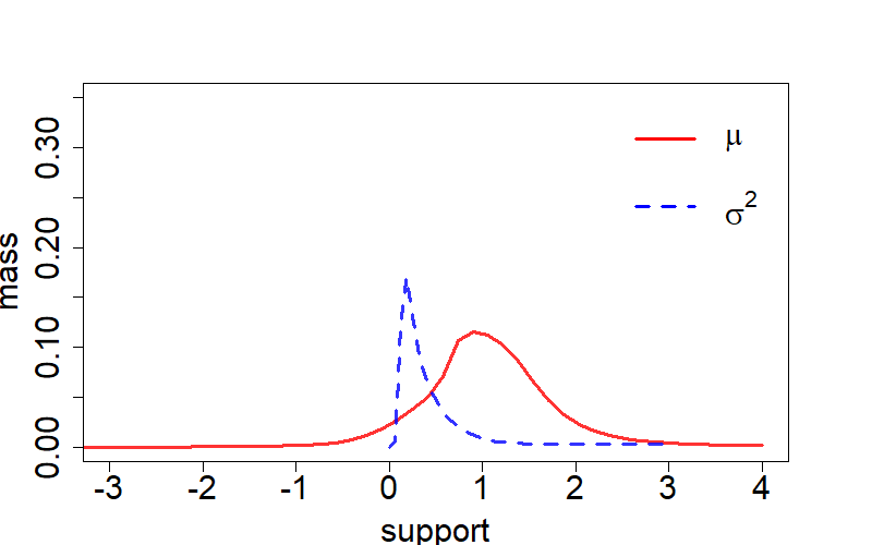
Example (3) : Bi-variate Gaussian location-scale mixture

In this case, we explore the application of bivariate neural-g in a Gaussion location-scale mixture model: $\pi(\mu,\sigma^2) \sim \text{Normal-inverse-gamma}(\mu=1,\sigma=1,\text{shape}=2,\text{scale}=0.5)$.

Seed <- 128783;set.seed(Seed);dist <- "Gaussian2s";param <- 0.5
n <- 1000;L <- 5;num_it <- 4000;n_grid <- 50;p <- 2
mu <- 1;sigma <- 1; shape <- 2;scale <- 0.5
Y <- matrix(0, n, p)
theta1 <- MCMCpack::rinvgamma(n, shape, scale)
theta2 <- rnorm(n, mu, sd = sqrt(theta1 * sigma^2))
for(i in 1:n){Y[i,] <- theta2[i]+theta1[i]*rnorm(p)}
net_g <- neural_g2(Y=Y, param=param, dist=dist, n=n, num_it=num_it, n_grid=n_grid, p=p)
mu_support <- unique(net_g$support[,1])
sig_support <- unique(net_g$support[,2])
mu_prob <- rep(0, n_grid);sigma_prob <- rep(0, n_grid)
for(i in 1:n_grid){
     mu_prob[i] <- sum( net_g$prob[net_g$support[,1]==mu_support[i]] )
     sigma_prob[i] <- sum( net_g$prob[net_g$support[,2]==sig_support[i]] )
}
plot(mu_support, mu_prob, col=rgb(1,0,0,0.8), type='l', xlim=c(-3,4),
     xlab='support', ylab='mass', lwd=3, ylim=c(0,0.35), cex.axis=1.85, cex.lab=1.85)
lines(sig_support, sigma_prob, col=rgb(0,0,1,0.8), type='l', lwd=3, lty=2)
legend(x=2.0, y=0.385, c(expression(mu),expression(sigma^2)),
       col=c(rgb(1,0,0),rgb(0,0,1)), lty=c(1,2), lwd=c(3,3),
       bty="n", x.intersp=0.5, y.intersp=0.8, seg.len=1.0, cex=1.85)

shijiew97 / neuralG