![]()
See scikit-hep/uproot4 for the latest version of Uproot. Old and new versions are available as separate packages,
because the interface has changed.
You can adopt the new library gradually by importing both in Python, switching to the old version as a contingency (missing feature or bug in the new version). Note that Uproot 3 returns old-style Awkward 0 arrays and Uproot 4 returns new-style Awkward 1 arrays. (The new version of Uproot was motivated by the new version of Awkward, to make a clear distinction.)
ROOT I/O in pure Python and Numpy.
uproot (originally μproot, for "micro-Python ROOT") is a reader and a writer of the ROOT file format using only Python and Numpy. Unlike the standard C++ ROOT implementation, uproot is only an I/O library, primarily intended to stream data into machine learning libraries in Python. Unlike PyROOT and root_numpy, uproot does not depend on C++ ROOT. Instead, it uses Numpy to cast blocks of data from the ROOT file as Numpy arrays.
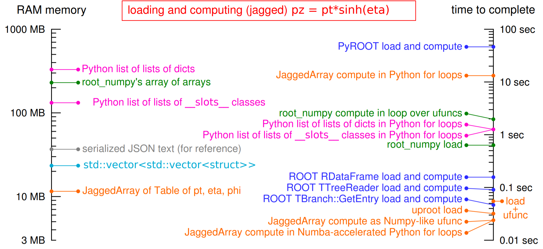
Python does not necessarily mean slow. As long as the data blocks ("baskets") are large, this "array at a time" approach can even be faster than "event at a time" C++. Below, the rate of reading data into arrays with uproot is shown to be faster than C++ ROOT (left) and root_numpy (right), as long as the baskets are tens of kilobytes or larger (for a variable number of muons per event in an ensemble of different physics samples; higher is better).
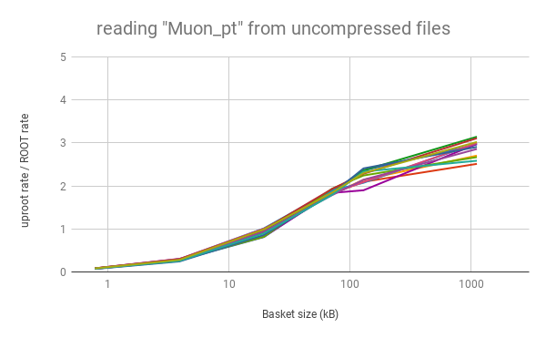 | 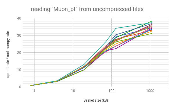 |
uproot is not maintained by the ROOT project team, so post bug reports here as GitHub issues, not on a ROOT forum. Thanks!
Install uproot like any other Python package:
The pip installer automatically installs strict dependencies; the conda installer also installs optional dependencies (except for Pandas).
- numpy (1.13.1+)
- Awkward Array 0.x
- uproot3-methods
- cachetools
- lz4 to read/write lz4-compressed ROOT files
- xxhash to read/write lz4-compressed ROOT files
- lzma to read/write lzma-compressed ROOT files in Python 2
- xrootd to access remote files through XRootD
- requests to access remote files through HTTP
- pandas to fill Pandas DataFrames instead of Numpy arrays
Reminder: you do not need C++ ROOT to run uproot.
If you have a question about how to use uproot that is not answered in the document below, I recommend asking your question on StackOverflow with the [uproot] tag. (I get notified of questions with this tag.) Note that this tag is primarily intended for the new version of Uproot, so if you're using this version (Uproot 3.x), be sure to mention that.
If you believe you have found a bug in uproot, post it on the GitHub issues tab.
Tutorial contents:
- Introduction
- What is uproot?
- Exploring a file
- Reading arrays from a TTree
- Caching data
- Lazy arrays
- Iteration
- Changing the output container type
- Filling Pandas DataFrames
- Selecting and interpreting branches
- TBranch interpretations
- Reading data into a preexisting array
- Passing many new interpretations in one call
- Multiple values per event: fixed size arrays
- Multiple values per event: leaf-lists
- Multiple values per event: jagged arrays
- Jagged array performance
- Special physics objects: Lorentz vectors
- Variable-width values: strings
- Arbitrary objects in TTrees
- Doubly nested jagged arrays (i.e. std::vector<std::vector<T>>) <#doubly-nested-jagged-arrays-ie-stdvectorstdvectort>__
- Parallel array reading
- Histograms, TProfiles, TGraphs, and others
- Creating and writing data to ROOT files
This tutorial is designed to help you start using uproot.
The original tutorial has been archived—this version was written in June 2019 in response to feedback from a series of tutorials I presented early this year and common questions in the GitHub issues. The new tutorial is executable on Binder and may be read in any order, though it has to be executed from top to bottom because some variables are reused.
Uproot is a Python package; it is pip and conda-installable, and it only depends on other Python packages. Although it is similar in function to root_numpy and root_pandas, it does not compile into ROOT and therefore avoids issues in which the version used in compilation differs from the version encountered at runtime.
In short, you should never see a segmentation fault.
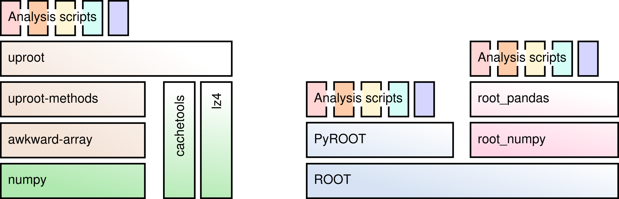
Uproot is strictly concerned with file I/O only—all other functionality is handled by other libraries:
- uproot3-methods: physics methods for types read from ROOT files, such as histograms and Lorentz vectors. It is intended to be largely user-contributed (and is).
- awkward-array: array manipulation beyond Numpy. Several are encountered in this tutorial, particularly lazy arrays and jagged arrays.
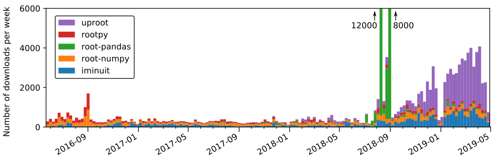
In the past year, uproot has become one of the most widely used Python packages made for particle physics, with users in all four LHC experiments, theory, neutrino experiments, XENON-nT (dark matter direct detection), MAGIC (gamma ray astronomy), and IceCube (neutrino astronomy).
uproot3.open is the entry point for reading a single file.
It takes a local filename path or a remote http:// or root:// URL. (HTTP requires the Python requests library and XRootD requires pyxrootd, both of which have to be explicitly pip-installed.)
import uproot3

file = uproot3.open("http://scikit-hep.org/uproot3/examples/nesteddirs.root")
file
# <ROOTDirectory b'tests/nesteddirs.root' at 0x7f37504ecc50>
uproot3.open returns a ROOTDirectory, which behaves like a Python dict; it has keys(), values(), and key-value access with square brackets.
file.keys()
# [b'one;1', b'three;1']

file["one"]
# <ROOTDirectory b'one' at 0x7f3750588710>
Subdirectories also have type ROOTDirectory, so they behave like Python dicts, too.
file["one"].keys()
# [b'two;1', b'tree;1']

file["one"].values()
# [<ROOTDirectory b'two' at 0x7f3750588fd0>, <TTree b'tree' at 0x7f3750588cc0>]
What’s the `b` before each object name? Python 3 distinguishes between bytestrings and encoded strings. ROOT object names have no encoding, such as Latin-1 or Unicode, so Uproot presents them as raw bytestrings. However, if you enter a Python string (no b) and it matches an object name (interpreted as plain ASCII), it will count as a match, as "one" does above.
What’s the `;1` after each object name? ROOT objects are versioned with a “cycle number.” If multiple objects are written to the ROOT file with the same name, they will have different cycle numbers, with the largest value being last. If you don’t specify a cycle number, you’ll get the latest one.
This file is deeply nested, so while you could find the TTree with
file["one"]["two"]["tree"]
# <TTree b'tree' at 0x7f37581297f0>
you can also find it using a directory path, with slashes.
file["one/two/tree"]
# <TTree b'tree' at 0x7f37504e4748>
Here are a few more tricks for finding your way around a file:
- the
keys(),values(), anditems()methods haveallkeys(),allvalues(),allitems()variants that recursively search through all subdirectories; - all of these functions can be filtered by name or class: see
ROOTDirectory.keys.
Here’s how you would search the subdirectories to find all TTrees:
file.allkeys(filterclass=lambda cls: issubclass(cls, uproot3.tree.TTreeMethods))
# [b'one/two/tree;1', b'one/tree;1', b'three/tree;1']
Or get a Python dict of them:
all_ttrees = dict(file.allitems(filterclass=lambda cls: issubclass(cls, uproot3.tree.TTreeMethods)))
all_ttrees
# {b'one/two/tree;1': <TTree b'tree' at 0x7f37504f85f8>,
#  b'one/tree;1': <TTree b'tree' at 0x7f37504f8710>,
#  b'three/tree;1': <TTree b'tree' at 0x7f37504f8470>}
Be careful: Python 3 is not as forgiving about matching key names. all_ttrees is a plain Python dict, so the key must be a bytestring and must include the cycle number.
all_ttrees[b"one/two/tree;1"]
# <TTree b'tree' at 0x7f37504f85f8>Objects in ROOT files can be uncompressed, compressed with ZLIB, compressed with LZMA, or compressed with LZ4. Uproot picks the right decompressor and gives you the objects transparently: you don’t have to specify anything. However, if an object is compressed with LZ4 and you don’t have the lz4 library installed, you’ll get an error with installation instructions in the message. ZLIB is part of the Python Standard Library, and LZMA is part of the Python 3 Standard Library, so you won’t get error messages about these except for LZMA in Python 2 (for which there is backports.lzma).
The ROOTDirectory class has a compression property that tells you the compression algorithm and level associated with this file,
file.compression
# <Compression 'zlib' 1>
but any object can be compressed with any algorithm at any level—this is only the default compression for the file. Some ROOT files are written with each TTree branch compressed using a different algorithm and level.
TTrees are special objects in ROOT files: they contain most of the physics data. Uproot presents TTrees as subclasses of TTreeMethods.
(Why subclass? Different ROOT files can have different versions of a class, so Uproot generates Python classes to fit the data, as needed. All TTrees inherit from TTreeMethods so that they get the same data-reading methods.)
events = uproot3.open("http://scikit-hep.org/uproot3/examples/Zmumu.root")["events"]
events
# <TTree b'events' at 0x7f375051fc18>
Although TTreeMethods objects behave like Python dicts of TBranchMethods objects, the easiest way to browse a TTree is by calling its show() method, which prints the branches and their interpretations as arrays.
events.keys()
# [b'Type', b'Run', b'Event', b'E1', b'px1', b'py1', b'pz1', b'pt1', b'eta1', b'phi1', b'Q1',
#  b'E2', b'px2', b'py2', b'pz2', b'pt2', b'eta2', b'phi2', b'Q2', b'M']
events.show()
# Type (no streamer) asstring()
# Run (no streamer) asdtype('>i4')
# Event (no streamer) asdtype('>i4')
# E1 (no streamer) asdtype('>f8')
# px1 (no streamer) asdtype('>f8')
# py1 (no streamer) asdtype('>f8')
# pz1 (no streamer) asdtype('>f8')
# pt1 (no streamer) asdtype('>f8')
# eta1 (no streamer) asdtype('>f8')
# phi1 (no streamer) asdtype('>f8')
# Q1 (no streamer) asdtype('>i4')
# E2 (no streamer) asdtype('>f8')
# px2 (no streamer) asdtype('>f8')
# py2 (no streamer) asdtype('>f8')
# pz2 (no streamer) asdtype('>f8')
# pt2 (no streamer) asdtype('>f8')
# eta2 (no streamer) asdtype('>f8')
# phi2 (no streamer) asdtype('>f8')
# Q2 (no streamer) asdtype('>i4')
# M (no streamer) asdtype('>f8')Basic information about the TTree, such as its number of entries, are available as properties.
events.name, events.title, events.numentries
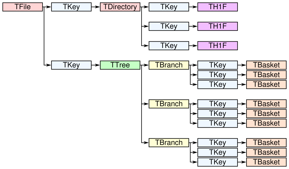
# (b'events', b'Z -> mumu events', 2304)ROOT files contain objects internally referred to via TKeys (dict-like lookup in Uproot). TTree organizes data in TBranches, and Uproot interprets one TBranch as one array, either a Numpy array or an Awkward Array. TBranch data are stored in chunks called TBaskets, though Uproot hides this level of granularity unless you dig into the details.
The bulk data in a TTree are not read until requested. There are many ways to do that:
- select a TBranch and call
TBranchMethods.array; - call
TTreeMethods.arraydirectly from the TTree object; - call
TTreeMethods.arraysto get several arrays at a time; - call
TBranch.lazyarray,TTreeMethods.lazyarray,TTreeMethods.lazyarrays, oruproot3.lazyarraysto get array-like objects that read on demand; - call
TTreeMethods.iterateoruproot3.iterateto explicitly iterate over chunks of data (to avoid reading more than would fit into memory); - call
TTreeMethods.pandasoruproot3.pandas.iterateto get Pandas DataFrames (Pandas must be installed).
Let’s start with the simplest.
a = events.array("E1")
a
# array([82.20186639, 62.34492895, 62.34492895, ..., 81.27013558, 81.27013558, 81.56621735])Since array is singular, you specify one branch name and get one array back. This is a Numpy array of 8-byte floating point numbers, the Numpy dtype specified by the "E1" branch’s interpretation.
events["E1"].interpretation
# asdtype('>f8')We can use this array in Numpy calculations; see the Numpy documentation for details.
import numpy
numpy.log(a)
# array([4.40917801, 4.13268234, 4.13268234, ..., 4.39777861, 4.39777861, 4.40141517])Numpy arrays are also the standard container for entering data into machine learning frameworks; see this Keras introduction, PyTorch introduction, TensorFlow introduction, or Scikit-Learn introduction to see how to put Numpy arrays to work in machine learning.
The TBranchMethods.array method is the same as TTreeMethods.array except that you don’t have to specify the TBranch name (naturally). Sometimes one is more convenient, sometimes the other.
events.array("E1"), events["E1"].array()
# (array([82.20186639, 62.34492895, 62.34492895, ..., 81.27013558, 81.27013558, 81.56621735]),
# array([82.20186639, 62.34492895, 62.34492895, ..., 81.27013558, 81.27013558, 81.56621735]))The plural arrays method is different. Whereas singular array could only return one array, plural arrays takes a list of names (possibly including wildcards) and returns them all in a Python dict.
events.arrays(["px1", "py1", "pz1"])
# {b'px1': array([-41.1952876, 35.1180497, 35.1180497, ..., 32.3774919, 32.377492, 32.4853938]),
# b'py1': array([ 17.4332439, -16.5703623, -16.5703623, ..., 1.1994057, 1.199405, 1.2013503]),
# b'pz1': array([-68.9649618, -48.7752465, -48.7752465, ..., -74.5324306, -74.532430, -74.8083724])}
events.arrays(["p[xyz]*"])
# {b'px1': array([-41.1952876, 35.1180497, 35.1180497, ..., 32.377491, 32.37749, 32.485393]),
# b'py1': array([ 17.4332439, -16.5703623, -16.5703623, ..., 1.199405, 1.19940, 1.201350]),
# b'pz1': array([-68.9649618, -48.7752465, -48.7752465, ..., -74.532430, -74.53243, -74.808372]),
# b'px2': array([ 34.1444372, -41.1952876, -40.8833234, ..., -68.041914, -68.79413, -68.794136]),
# b'py2': array([-16.1195245, 17.4332439, 17.2992970, ..., -26.105847, -26.39840, -26.398400]),
# b'pz2': array([ -47.426984, -68.9649618, -68.4472551, ..., -152.235018, -153.84760, -153.847603])}As with all ROOT object names, the TBranch names are bytestrings (prepended by b). If you know the encoding or it doesn’t matter ("ascii" and "utf-8" are generic), pass a namedecode to get keys that are strings.
events.arrays(["p[xyz]*"], namedecode="utf-8")
# {'px1': array([-41.1952876, 35.1180497, 35.11804977, ..., 32.377491, 32.377491, 32.485393]),
# 'py1': array([ 17.4332439, -16.5703623, -16.57036233, ..., 1.199405, 1.199405, 1.201350]),
# 'pz1': array([-68.9649618, -48.7752465, -48.77524654, ..., -74.532430, -74.532430, -74.808372]),
# 'px2': array([ 34.1444372, -41.1952876, -40.88332344, ..., -68.041914, -68.794136, -68.794136]),
# 'py2': array([-16.1195245, 17.4332439, 17.29929704, ..., -26.105847, -26.398400, -26.398400]),
# 'pz2': array([-47.4269843, -68.9649618, -68.44725519, ..., -152.235018, -153.847603, -153.847603])}These array-reading functions have many parameters, but most of them have the same names and meanings across all the functions. Rather than discuss all of them here, they’ll be presented in context in sections on special features below.
Every time you ask for arrays, Uproot goes to the file and re-reads them. For especially large arrays, this can take a long time.
For quicker access, Uproot’s array-reading functions have a cache parameter, which is an entry point for you to manage your own cache. The cache only needs to behave like a dict (many third-party Python caches do).
mycache = {}
# first time: reads from file
events.arrays(["p[xyz]*"], cache=mycache);
# any other time: reads from cache
events.arrays(["p[xyz]*"], cache=mycache);In this example, the cache is a simple Python dict. Uproot has filled it with unique ID → array pairs, and it uses the unique ID to identify an array that it has previously read. You can see that it’s full by looking at those keys:
mycache
# {'AAGUS3fQmKsR56dpAQAAf77v;events;px1;asdtype(Bf8(),Lf8());0-2304':
# array([-41.19528764, 35.11804977, 35.11804977, ..., 32.37749196, 32.37749196, 32.48539387]),
# 'AAGUS3fQmKsR56dpAQAAf77v;events;py1;asdtype(Bf8(),Lf8());0-2304':
# array([ 17.4332439 , -16.57036233, -16.57036233, ..., 1.19940578, 1.19940578, 1.2013503 ]),
# 'AAGUS3fQmKsR56dpAQAAf77v;events;pz1;asdtype(Bf8(),Lf8());0-2304':
# array([-68.96496181, -48.77524654, -48.77524654, ..., -74.53243061, -74.53243061, -74.80837247]),
# 'AAGUS3fQmKsR56dpAQAAf77v;events;px2;asdtype(Bf8(),Lf8());0-2304':
# array([ 34.14443725, -41.19528764, -40.88332344, ..., -68.04191497, -68.79413604, -68.79413604]),
# 'AAGUS3fQmKsR56dpAQAAf77v;events;py2;asdtype(Bf8(),Lf8());0-2304':
# array([-16.11952457, 17.4332439 , 17.29929704, ..., -26.10584737, -26.39840043, -26.39840043]),
# 'AAGUS3fQmKsR56dpAQAAf77v;events;pz2;asdtype(Bf8(),Lf8());0-2304':
# array([ -47.4269843, -68.9649618, -68.4472551, ..., -152.2350181, -153.8476038, -153.8476038])
# }though they’re not very human-readable.
If you’re running out of memory, you could manually clear your cache by simply clearing the dict.
mycache.clear()
mycache
# {}Now the same line of code reads from the file again.
# not in cache: reads from file
events.arrays(["p[xyz]*"], cache=mycache)This manual process of clearing the cache when you run out of memory is not very robust. What you want instead is a dict-like object that drops elements on its own when memory is scarce.
Uproot has an ArrayCache class for this purpose, though it’s a thin wrapper around the third-party cachetools library. Whereas cachetools drops old data from cache when a maximum number of items is reached, ArrayCache drops old data when the data usage reaches a limit, specified in bytes.
mycache = uproot3.ArrayCache("100 kB")
events.arrays("*", cache=mycache);
len(mycache), len(events.keys())
# (6, 20)With a limit of 100 kB, only 6 of the 20 arrays fit into cache, the rest have been evicted.
All data sizes in Uproot are specified as an integer in bytes (integers) or a string with the appropriate unit (interpreted as powers of 1024, not 1000).
The fact that any dict-like object may be a cache opens many possibilities. If you’re struggling with a script that takes a long time to load data, then crashes, you may want to try a process-independent cache like memcached. If you have a small, fast disk, you may want to consider diskcache to temporarily hold arrays from ROOT files on the big, slow disk.
All of the array-reading functions have a cache parameter to accept a cache object. This is the high-level cache, which caches data after it has been fully interpreted. These functions also have a basketcache parameter to cache data after reading and decompressing baskets, but before interpretation as high-level arrays. The main purpose of this is to avoid reading TBaskets twice when an iteration step falls in the middle of a basket (see below). There is also a keycache for caching ROOT’s TKey objects, which use negligible memory but would be a bottleneck to re-read when TBaskets are provided by a basketcache.
At the lowest level of abstraction, raw bytes are cached by the HTTP and XRootD remote file readers. You can control the memory remote file memory use with uproot3.HTTPSource.defaults["limitbytes"] and uproot3.XRootDSource.defaults["limitbytes"], either by globally setting these parameters before opening a file, or by passing them to uproot3.open through the limitbytes parameter.
# default remote file caches in MB
uproot3.HTTPSource.defaults["limitbytes"] / 1024**2, uproot3.XRootDSource.defaults["limitbytes"] / 1024**2
# (32.0, 32.0)If you want to limit this cache to less than the default chunkbytes of 1 MB, be sure to make the chunkbytes smaller, so that it’s able to load at least one chunk!
uproot3.open("http://scikit-hep.org/uproot3/examples/Zmumu.root", limitbytes="100 kB", chunkbytes="10 kB")
# <ROOTDirectory b'Zmumu.root' at 0x7f375041f278>By default (unless localsource is overridden), local files are memory-mapped, so the operating system manages its byte-level cache.
If you call TBranchMethods.array, TTreeMethods.array, or TTreeMethods.arrays, Uproot reads the file or cache immediately and returns an in-memory array. For exploratory work or to control memory usage, you might want to let the data be read on demand.
The TBranch.lazyarray, TTreeMethods.lazyarray, TTreeMethods.lazyarrays, and uproot.lazyarrays functions take most of the same parameters but return lazy array objects, rather than Numpy arrays.
data = events.lazyarrays("*")
data
# <ChunkedArray [<Row 0> <Row 1> <Row 2> ... <Row 2301> <Row 2302> <Row 2303>] at 0x7f375041fa20>This ChunkedArray represents all the data in the file in chunks specified by ROOT’s internal baskets (specifically, the places where the baskets align, called “clusters”). Each chunk contains a VirtualArray, which is read when any element from it is accessed.
data = events.lazyarrays(entrysteps=500) # chunks of 500 events each
dataE1 = data["E1"]
dataE1
# <ChunkedArray [82.2018663875 62.3449289481 62.3449289481 ...
# 81.2701355756 81.2701355756 81.5662173543] at 0x7f3750467400>Requesting "E1" through all the chunks and printing it (above) has caused the first and last chunks of the array to be read, because that’s all that got written to the screen. (See the ...?)
[chunk.ismaterialized for chunk in dataE1.chunks]
# [True, False, False, False, True]These arrays can be used with Numpy’s universal functions (ufuncs), which are the mathematical functions that perform elementwise mathematics.
numpy.log(dataE1)
# <ChunkedArray [4.409178007248409 4.132682336791151 4.132682336791151 4.104655794838432
# 3.733527454020269 3.891440776178839 3.891440776178839 ...] at 0x7f37504560b8>Now all of the chunks have been read, because the values were needed to compute log(E1) for all E1.
[chunk.ismaterialized for chunk in dataE1.chunks]
# [True, True, True, True, True](Note: only ufuncs recognize these lazy arrays because Numpy provides a mechanism to override ufuncs but a similar mechanism for high-level functions is still in development. To turn lazy arrays into Numpy arrays, pass them to the Numpy constructor, as shown below. This causes the whole array to be loaded into memory and to be stitched together into a contiguous whole.)
numpy.array(dataE1)
# array([82.20186639, 62.34492895, 62.34492895, ..., 81.27013558,
# 81.27013558, 81.56621735])There’s a lazy version of each of the array-reading functions in TTreeMethods and TBranchMethods, but there’s also module-level uproot.lazyarray and uproot.lazyarrays. These functions let you make a lazy array that spans many files.
These functions may be thought of as alternatives to ROOT’s TChain: a TChain presents many files as though they were a single TTree, and a file-spanning lazy array presents many files as though they were a single array. See Iteration below as a more explicit TChain alternative.
data = uproot3.lazyarray(
# list of files; local files can have wildcards (*)
["http://scikit-hep.org/uproot3/examples/sample-%s-zlib.root" % x
for x in ["5.23.02", "5.24.00", "5.25.02", "5.26.00", "5.27.02", "5.28.00",
"5.29.02", "5.30.00", "6.08.04", "6.10.05", "6.14.00"]],
# TTree name in each file
"sample",
# branch(s) in each file for lazyarray(s)
"f8")
data
# <ChunkedArray [-14.9 -13.9 -12.9 ... 12.1 13.1 14.1] at 0x7f3739bc37f0>This data represents the entire set of files, and the only up-front processing that had to be done was to find out how many entries each TTree contains.
It uses the uproot3.numentries shortcut method (which reads less data than normal file-opening):
dict(uproot3.numentries(
# list of files; local files can have wildcards (*)
["http://scikit-hep.org/uproot3/examples/sample-%s-zlib.root" % x
for x in ["5.23.02", "5.24.00", "5.25.02", "5.26.00", "5.27.02", "5.28.00",
"5.29.02", "5.30.00", "6.08.04", "6.10.05", "6.14.00"]],
# TTree name in each file
"sample",
# total=True adds all values; total=False leaves them as a dict
total=False))
# {'http://scikit-hep.org/uproot3/examples/sample-5.23.02-zlib.root': 30,
# 'http://scikit-hep.org/uproot3/examples/sample-5.24.00-zlib.root': 30,
# 'http://scikit-hep.org/uproot3/examples/sample-5.25.02-zlib.root': 30,
# 'http://scikit-hep.org/uproot3/examples/sample-5.26.00-zlib.root': 30,
# 'http://scikit-hep.org/uproot3/examples/sample-5.27.02-zlib.root': 30,
# 'http://scikit-hep.org/uproot3/examples/sample-5.28.00-zlib.root': 30,
# 'http://scikit-hep.org/uproot3/examples/sample-5.29.02-zlib.root': 30,
# 'http://scikit-hep.org/uproot3/examples/sample-5.30.00-zlib.root': 30,
# 'http://scikit-hep.org/uproot3/examples/sample-6.08.04-zlib.root': 30,
# 'http://scikit-hep.org/uproot3/examples/sample-6.10.05-zlib.root': 30,
# 'http://scikit-hep.org/uproot3/examples/sample-6.14.00-zlib.root': 30}By default, lazy arrays hold onto all data that have been read as long as the lazy array continues to exist. To use a lazy array as a window into a very large dataset, you’ll have to limit how much it’s allowed to keep in memory at a time.
This is caching, and the caching mechanism is the same as before:
mycache = uproot3.cache.ArrayCache(100*1024) # 100 kB
data = events.lazyarrays(entrysteps=500, cache=mycache)
data
# <ChunkedArray [<Row 0> <Row 1> <Row 2> ... <Row 2301> <Row 2302> <Row 2303>] at 0x7f3739b90f28>Before performing a calculation, the cache is empty.
len(mycache)
# 0numpy.sqrt((data["E1"] + data["E2"])**2 - (data["px1"] + data["px2"])**2 -
(data["py1"] + data["py2"])**2 - (data["pz1"] + data["pz2"])**2)
# <ChunkedArray [82.46269155513643 83.62620400526137 83.30846466680981 82.14937288090277
# 90.46912303551746 89.75766317061574 89.77394317215372 ...] at 0x7f3739b9eda0>After performing the calculation, the cache contains only as many chunks as it could hold.
# chunks in cache chunks touched to compute (E1 + E2)**2 - (px1 + px2)**2 - (py1 + py2)**2 - (pz1 + pz2)**2
len(mycache), len(data["E1"].chunks) * 8
# (28, 40)The ChunkedArray and VirtualArray classes are defined in the Awkward Array library installed with Uproot. These arrays can be saved to files in a way that preserves their virtualness, which allows you to save a “diff” with respect to the original ROOT files.
Below, we load lazy arrays from a ROOT file with persistvirtual=True and add a derived feature:
data = events.lazyarrays(["E*", "p[xyz]*"], persistvirtual=True)
data["mass"] = numpy.sqrt((data["E1"] + data["E2"])**2 - (data["px1"] + data["px2"])**2 -
(data["py1"] + data["py2"])**2 - (data["pz1"] + data["pz2"])**2)and save the whole thing to an Awkward Array file (.awkd).
import awkward0
awkward0.save("derived-feature.awkd", data, mode="w")When we read it back, the derived features come from the Awkward Array file but the original features are loaded as pointers to the original ROOT files (VirtualArrays whose array-making function knows the original ROOT filenames—don’t move them!).
data2 = awkward0.load("derived-feature.awkd")
# reads from derived-feature.awkd
data2["mass"]
# <ChunkedArray [82.46269155513643 83.62620400526137 83.30846466680981 ...
# 95.96547966432459 96.49594381502096 96.6567276548945] at 0x7f3739bafc88>
# reads from the original ROOT flies
data2["E1"]
# <ChunkedArray [82.2018663875 62.3449289481 62.3449289481 ...
# 81.2701355756 81.2701355756 81.5662173543] at 0x7f3739b3e400>Similarly, a dataset with a cut applied saves the identities of the selected events but only pointers to the original ROOT data. This acts as a lightweight skim.
selected = data[data["mass"] < 80]
selected
# <ChunkedArray [<Row 16> <Row 17> <Row 18> <Row 19> <Row 47> <Row 48> <Row 49> ...] at 0x7f3739b3e7f0>
awkward0.save("selected-events.awkd", selected, mode="w")
data3 = awkward0.load("selected-events.awkd")
data3
# <ChunkedArray [<Row 16> <Row 17> <Row 18> ... <Row 2297> <Row 2298> <Row 2299>] at 0x7f3739b1e048>Dask is a framework for delayed and distributed computation with lazy array and dataframe interfaces. To turn Uproot’s lazy arrays into Dask objects, use the uproot3.daskarray and uproot3.daskframe functions.
uproot3.daskarray("http://scikit-hep.org/uproot3/examples/Zmumu.root", "events", "E1")
# dask.array<array, shape=(2304,), dtype=float64, chunksize=(2304,)>uproot3.daskframe("http://scikit-hep.org/uproot3/examples/Zmumu.root", "events")| Type | Run | Event | E1 | px1 | py1 | pz1 | pt1 | eta1 | phi1 | Q1 | E2 | px2 | py2 | pz2 | pt2 | eta2 | phi2 | Q2 | M | |
|---|---|---|---|---|---|---|---|---|---|---|---|---|---|---|---|---|---|---|---|---|
| npartitions=1 | ||||||||||||||||||||
| 0 | object | int32 | int32 | float64 | float64 | float64 | float64 | float64 | float64 | float64 | int32 | float64 | float64 | float64 | float64 | float64 | float64 | float64 | int32 | float64 |
| 2303 | ... | ... | ... | ... | ... | ... | ... | ... | ... | ... | ... | ... | ... | ... | ... | ... | ... | ... | ... | ... |
Lazy arrays implicitly step through chunks of data to give you the impression that you have a larger array than memory can hold all at once. The next two methods explicitly step through chunks of data, to give you more control over the process.
TTreeMethods.iterate iterates over chunks of a TTree and uproot3.iterate iterates through files.
Like a file-spanning lazy array, a file-spanning iterator erases the difference between files and may be used as a TChain alternative. However, the iteration is over chunks of many events, not single events.
histogram = None
for data in events.iterate(["E*", "p[xyz]*"], namedecode="utf-8"):
# operate on a batch of data in the loop
mass = numpy.sqrt((data["E1"] + data["E2"])**2 - (data["px1"] + data["px2"])**2 -
(data["py1"] + data["py2"])**2 - (data["pz1"] + data["pz2"])**2)
# accumulate results
counts, edges = numpy.histogram(mass, bins=120, range=(0, 120))
if histogram is None:
histogram = counts, edges
else:
histogram = histogram[0] + counts, edgesimport matplotlib.pyplot
counts, edges = histogram
matplotlib.pyplot.step(x=edges, y=numpy.append(counts, 0), where="post");
matplotlib.pyplot.xlim(edges[0], edges[-1]);
matplotlib.pyplot.ylim(0, counts.max() * 1.1);
matplotlib.pyplot.xlabel("mass");
matplotlib.pyplot.ylabel("events per bin");
This differs from the lazy array approach in that you need to explicitly manage the iteration, as in this histogram accumulation. However, since we aren’t caching, the previous array batch is deleted as soon as data goes out of scope, so it is easier to control which arrays are in memory and which aren’t.
Choose lazy arrays or iteration according to the degree of control you need.
uproot3.iterate crosses file boundaries as part of its iteration, and that’s information we might need in the loop. If the following are True, each step in iteration is a tuple containing the arrays and the additional information.
- reportpath: the full path or URL of the (possibly remote) file;
- reportfile: the
ROOTDirectoryobject itself (so that you don’t need to re-open it at each iteration step); - reportentries: the starting and stopping entry numbers for this chunk of data. In a multi-file iteration, these are global (always increasing, not returning to zero as we start the next file).
for path, file, start, stop, arrays in uproot3.iterate(
["http://scikit-hep.org/uproot3/examples/sample-%s-zlib.root" % x
for x in ["5.23.02", "5.24.00", "5.25.02", "5.26.00", "5.27.02", "5.28.00",
"5.29.02", "5.30.00", "6.08.04", "6.10.05", "6.14.00"]],
"sample",
"f8",
reportpath=True, reportfile=True, reportentries=True):
print(path, file, start, stop, len(arrays))
# http://scikit-hep.org/uproot3/examples/sample-5.23.02-zlib.root
# <ROOTDirectory b'sample-5.23.02-zlib.root' at 0x7f36441c3c50> 0 30 1
# http://scikit-hep.org/uproot3/examples/sample-5.24.00-zlib.root
# <ROOTDirectory b'sample-5.24.00-zlib.root' at 0x7f364418e8d0> 30 60 1
# http://scikit-hep.org/uproot3/examples/sample-5.25.02-zlib.root
# <ROOTDirectory b'sample-5.25.02-zlib.root' at 0x7f36441034e0> 60 90 1
# http://scikit-hep.org/uproot3/examples/sample-5.26.00-zlib.root
# <ROOTDirectory b'sample-5.26.00-zlib.root' at 0x7f3644095f98> 90 120 1
# http://scikit-hep.org/uproot3/examples/sample-5.27.02-zlib.root
# <ROOTDirectory b'sample-5.27.02-zlib.root' at 0x7f36440c4c88> 120 150 1
# http://scikit-hep.org/uproot3/examples/sample-5.28.00-zlib.root
# <ROOTDirectory b'sample-5.28.00-zlib.root' at 0x7f3644083898> 150 180 1
# http://scikit-hep.org/uproot3/examples/sample-5.29.02-zlib.root
# <ROOTDirectory b'sample-5.29.02-zlib.root' at 0x7f36440765c0> 180 210 1
# http://scikit-hep.org/uproot3/examples/sample-5.30.00-zlib.root
# <ROOTDirectory b'sample-5.30.00-zlib.root' at 0x7f36440dec88> 210 240 1
# http://scikit-hep.org/uproot3/examples/sample-6.08.04-zlib.root
# <ROOTDirectory b'sample-6.08.04-zlib.root' at 0x7f364418e550> 240 270 1
# http://scikit-hep.org/uproot3/examples/sample-6.10.05-zlib.root
# <ROOTDirectory b'sample-6.10.05-zlib.root' at 0x7f36441b76a0> 270 300 1
# http://scikit-hep.org/uproot3/examples/sample-6.14.00-zlib.root
# <ROOTDirectory b'sample-6.14.00-zlib.root' at 0x7f3644128cf8> 300 330 1All array-reading functions have the following parameters:
- entrystart: the first entry to read, by default
0; - entrystop: one after the last entry to read, by default
numentries.
Setting entrystart and/or entrystop differs from slicing the resulting array in that slicing reads, then discards, but these parameters minimize the data to read.
len(events.array("E1", entrystart=100, entrystop=300))
# 200As with Python slices, the entrystart and entrystop can be negative to count from the end of the TTree.
events.array("E1", entrystart=-10)
# array([ 35.36458334, 35.46037568, 27.74254176, 32.67634359,
# 32.67634359, 32.70165023, 168.78012134, 81.27013558,
# 81.27013558, 81.56621735])Internally, ROOT files are written in chunks and whole chunks must be read, so the best places to set entrystart and entrystop are between basket boundaries.
# This file has small TBaskets
tree = uproot3.open("http://scikit-hep.org/uproot3/examples/foriter.root")["foriter"]
branch = tree["data"]
[branch.basket_numentries(i) for i in range(branch.numbaskets)]
# [6, 6, 6, 6, 6, 6, 6, 4]# (entrystart, entrystop) pairs where ALL the TBranches' TBaskets align
list(tree.clusters())
# [(0, 6), (6, 12), (12, 18), (18, 24), (24, 30), (30, 36), (36, 42), (42, 46)]Or simply,
branch.baskets()
# [array([0, 1, 2, 3, 4, 5], dtype=int32),
# array([ 6, 7, 8, 9, 10, 11], dtype=int32),
# array([12, 13, 14, 15, 16, 17], dtype=int32),
# array([18, 19, 20, 21, 22, 23], dtype=int32),
# array([24, 25, 26, 27, 28, 29], dtype=int32),
# array([30, 31, 32, 33, 34, 35], dtype=int32),
# array([36, 37, 38, 39, 40, 41], dtype=int32),
# array([42, 43, 44, 45], dtype=int32)]In addition to entrystart and entrystop, the lazy array and iteration functions also have:
- entrysteps: the number of entries to read in each chunk or step,
numpy.inffor make the chunks/steps as big as possible (limited by file boundaries), a memory size string, or a list of(entrystart, entrystop)pairs to be explicit.
[len(chunk) for chunk in events.lazyarrays(entrysteps=500)["E1"].chunks]
# [500, 500, 500, 500, 304][len(data[b"E1"]) for data in events.iterate(["E*", "p[xyz]*"], entrysteps=500)]
# [500, 500, 500, 500, 304]The TTree lazy array/iteration functions (TTreeMethods.array, TTreeMethods.arrays, TBranch.lazyarray, TTreeMethods.lazyarray, and TTreeMethods.lazyarrays) use basket or cluster sizes as a default entrysteps, while multi-file lazy array/iteration functions (uproot3.lazyarrays and uproot3.iterate) use the maximum per file: numpy.inf.
# This file has small TBaskets
tree = uproot3.open("http://scikit-hep.org/uproot3/examples/foriter.root")["foriter"]
branch = tree["data"]
[len(a["data"]) for a in tree.iterate(namedecode="utf-8")]
# [6, 6, 6, 6, 6, 6, 6, 4]# This file has small TBaskets
[len(a["data"]) for a in uproot3.iterate(["http://scikit-hep.org/uproot3/examples/foriter.root"] * 3,
"foriter", namedecode="utf-8")]
# [46, 46, 46]One particularly useful way to specify the entrysteps is with a memory size string. This string consists of a number followed by a memory unit: B for bytes, kB for kilobytes, MB, GB, and so on (whitespace and case insensitive).
The chunks are not guaranteed to fit the memory size perfectly or even be less than the target size. Uproot picks a fixed number of events that approximates this size on average. The result depends on the number of branches chosen because it is the total size of the set of branches that are chosen for the memory target.
[len(data[b"E1"]) for data in events.iterate(["E*", "p[xyz]*"], entrysteps="50 kB")]
# [753, 753, 753, 45][len(data[b"E1"]) for data in events.iterate(entrysteps="50 kB")]
# [359, 359, 359, 359, 359, 359, 150]Since lazy arrays represent all branches but we won’t necessarily be reading all branches, memory size chunking is less useful for lazy arrays, but you can do it because all function parameters are treated consistently.
[len(chunk) for chunk in events.lazyarrays(entrysteps="50 kB")["E1"].chunks]
# [359, 359, 359, 359, 359, 359, 150]Since iteration gives you more precise control over which set of events you’re processing at a given time, caching with the cache parameter is less useful than it is with lazy arrays. For consistency’s sake, the TTreeMethods.iterate and uproot3.iterate functions provide a cache parameter and it works the same way that it does in other array-reading functions, but its effect would be to retain the previous step’s arrays while working on a new step in the iteration. Presumably, the reason you’re iterating is because only the current step fits into memory, so this is not a useful feature.
However, the basketcache is very useful for iteration, more so than it is for lazy arrays. If an iteration step falls in the middle of a TBasket, the whole TBasket must be read in that step, despite the fact that only part of it is incorporated into the output array. The remainder of the TBasket will be used in the next iteration step, so caching it for exactly one iteration step is ideal: it avoids the need to reread it and decompress it again.
It is such a useful feature that it’s built into TTreeMethods.iterate and uproot3.iterate by default. If you don’t set a basketcache, these functions will create one with no memory limit and save TBaskets in it for exactly one iteration step, eliminating that temporary cache at the end of iteration. (The same is true of the keycache.)
Thus, you probably don’t want to set any explicit caches while iterating. Setting an explicit basketcache would introduce an upper limit on how much it can store, but it would lose the property of evicting after exactly one iteration step (because the connection between the cache object and the iterator would be lost). If you’re running out of memory during iteration, try reducing the entrysteps.
When we ask for TTreeMethods.arrays (plural), TTreeMethods.iterate, or uproot3.iterate, we get a Python dict mapping branch names to arrays. (As a reminder, namedecode=“utf-8” makes those branch names Python strings, rather than bytestrings.) Sometimes, we want a different kind of container.
- outputtype: the type of the container to hold the output arrays.
One particularly useful container is tuple, which can be unpacked by a tuple-assignment.
px, py, pz = events.arrays("p[xyz]1", outputtype=tuple)px
# array([-41.19528764, 35.11804977, 35.11804977, ..., 32.37749196,
# 32.37749196, 32.48539387])Using tuple as an outputtype in TTreeMethods.iterate and uproot3.iterate lets us unpack the arrays in Python’s for statement.
for px, py, pz in events.iterate("p[xyz]1", outputtype=tuple):
px**2 + py**2 + pz**2Another useful type is collections.namedtuple, which packs everything into a single object, but the fields are accessible by name.
import collections # from the Python standard library
a = events.arrays("p[xyz]1", outputtype=collections.namedtuple)a.px1
# array([-41.19528764, 35.11804977, 35.11804977, ..., 32.37749196,
# 32.37749196, 32.48539387])You can also use your own classes.
class Stuff:
def __init__(self, px, py, pz):
self.p = numpy.sqrt(px**2 + py**2 + pz**2)
def __repr__(self):
return "<Stuff %r>" % self.p
events.arrays("p[xyz]1", outputtype=Stuff)
# <Stuff array([82.20179848, 62.34483942, 62.34483942, ..., 81.27006689,
# 81.27006689, 81.56614892])>And perhaps most importantly, you can pass in pandas.DataFrame.
import pandas
events.arrays("p[xyz]1", outputtype=pandas.DataFrame, entrystop=10)| px1 | py1 | pz1 | |
|---|---|---|---|
| entry | |||
| 0 | -41.195288 | 17.433244 | -68.964962 |
| 1 | 35.118050 | -16.570362 | -48.775247 |
| 2 | 35.118050 | -16.570362 | -48.775247 |
| 3 | 34.144437 | -16.119525 | -47.426984 |
| 4 | 22.783582 | 15.036444 | -31.689894 |
| 5 | -19.862307 | -9.204225 | 43.817098 |
| 6 | -19.862307 | -9.204225 | 43.817098 |
| 7 | -20.177373 | -9.354149 | 44.513955 |
| 8 | 71.143711 | 29.542308 | -108.150553 |
| 9 | 51.050486 | -51.849400 | -49.631328 |
The previous example filled a pandas.DataFrame by explicitly passing it as an outputtype. Pandas is such an important container type that there are specialized functions for it: TTreeMethods.pandas.df and uproot3.pandas.df.
events.pandas.df("p[xyz]1", entrystop=10)| px1 | py1 | pz1 | |
|---|---|---|---|
| entry | |||
| 0 | -41.195288 | 17.433244 | -68.964962 |
| 1 | 35.118050 | -16.570362 | -48.775247 |
| 2 | 35.118050 | -16.570362 | -48.775247 |
| 3 | 34.144437 | -16.119525 | -47.426984 |
| 4 | 22.783582 | 15.036444 | -31.689894 |
| 5 | -19.862307 | -9.204225 | 43.817098 |
| 6 | -19.862307 | -9.204225 | 43.817098 |
| 7 | -20.177373 | -9.354149 | 44.513955 |
| 8 | 71.143711 | 29.542308 | -108.150553 |
| 9 | 51.050486 | -51.849400 | -49.631328 |
The entry index in the resulting DataFrame represents the actual entry numbers in the file. For instance, counting from the end:
events.pandas.df("p[xyz]1", entrystart=-10)| px1 | py1 | pz1 | |
|---|---|---|---|
| entry | |||
| 2294 | 12.966984 | 30.974506 | 11.094139 |
| 2295 | 13.001270 | 31.059021 | 11.123455 |
| 2296 | -16.891371 | -15.335677 | -15.784044 |
| 2297 | 19.037577 | 14.820723 | 22.037447 |
| 2298 | 19.037577 | 14.820723 | 22.037447 |
| 2299 | 19.054651 | 14.833954 | 22.051323 |
| 2300 | -68.041915 | -26.105847 | -152.235018 |
| 2301 | 32.377492 | 1.199406 | -74.532431 |
| 2302 | 32.377492 | 1.199406 | -74.532431 |
| 2303 | 32.485394 | 1.201350 | -74.808372 |
The uproot3.pandas.df function doesn’t have a reportentries because they’re included in the DataFrame itself.
for df in uproot3.pandas.iterate("http://scikit-hep.org/uproot3/examples/Zmumu.root", "events", "p[xyz]1",
entrysteps=500):
print(df[:3])
# px1 py1 pz1
# entry
# 0 -41.195288 17.433244 -68.964962
# 1 35.118050 -16.570362 -48.775247
# 2 35.118050 -16.570362 -48.775247
# px1 py1 pz1
# entry
# 500 39.163212 -19.185280 -13.979333
# 501 39.094970 -19.152964 -13.936115
# 502 -7.656437 -33.431880 91.840257
# px1 py1 pz1
# entry
# 1000 26.043759 -17.618814 -0.567176
# 1001 26.043759 -17.618814 -0.567176
# 1002 25.996204 -17.585241 -0.568920
# px1 py1 pz1
# entry
# 1500 82.816840 13.262734 27.797909
# 1501 -11.416911 39.815352 32.349893
# 1502 -11.416911 39.815352 32.349893
# px1 py1 pz1
# entry
# 2000 -43.378378 -15.235422 3.019698
# 2001 -43.378378 -15.235422 3.019698
# 2002 -43.244422 -15.187402 3.003985Part of the motivation for a special function is that it’s the first of potentially many external connectors (Dask is another: see above). The other part is that these functions have more Pandas-friendly default parameters, such as flatten=True.
Flattening turns multiple values per entry (i.e. multiple particles per event) into separate DataFrame rows, maintaining the nested structure in the DataFrame index. Flattening is usually undesirable for arrays—because arrays don’t have an index to record that information—but it’s usually desirable for DataFrames.
events2 = uproot3.open("http://scikit-hep.org/uproot3/examples/HZZ.root")["events"] # non-flat dataevents2.pandas.df(["MET_p*", "Muon_P*"], entrystop=10, flatten=False) # not the default| MET_px | MET_py | Muon_Px | Muon_Py | Muon_Pz | |
|---|---|---|---|---|---|
| entry | |||||
| 0 | 5.912771 | 2.563633 | [-52.899456, 37.73778] | [-11.654672, 0.6934736] | [-8.160793, -11.307582] |
| 1 | 24.765203 | -16.349110 | [-0.81645936] | [-24.404259] | [20.199968] |
| 2 | -25.785088 | 16.237131 | [48.98783, 0.8275667] | [-21.723139, 29.800508] | [11.168285, 36.96519] |
| 3 | 8.619896 | -22.786547 | [22.088331, 76.69192] | [-85.835464, -13.956494] | [403.84845, 335.0942] |
| 4 | 5.393139 | -1.310052 | [45.17132, 39.750957] | [67.24879, 25.403667] | [-89.69573, 20.115053] |
| 5 | -3.759475 | -19.417021 | [9.22811, -5.793715] | [40.55438, -30.295189] | [-14.642164, 42.954376] |
| 6 | 23.962149 | -9.049156 | [12.538717, 29.54184] | [-42.54871, -4.4455166] | [-124.44899, -26.356554] |
| 7 | -57.533348 | -20.487679 | [34.88376] | [-15.982724] | [155.53117] |
| 8 | 42.416195 | -94.350861 | [-53.166973, 11.49187] | [92.02971, -4.4173865] | [35.638836, -17.473787] |
| 9 | -1.914469 | -23.963034 | [-67.014854, -18.118755] | [53.159172, -35.106167] | [54.41294, 58.036896] |
DataFrames like the above are slow (the cell entries are Python lists) and difficult to use in Pandas. Pandas doesn’t have specialized functions for manipulating this kind of structure.
However, if we use the default flatten=True:
df = events2.pandas.df(["MET_p*", "Muon_P*"], entrystop=10)
df| MET_px | MET_py | Muon_Px | Muon_Py | Muon_Pz | ||
|---|---|---|---|---|---|---|
| entry | subentry | |||||
| 0 | 0 | 5.912771 | 2.563633 | -52.899456 | -11.654672 | -8.160793 |
| 1 | 5.912771 | 2.563633 | 37.737782 | 0.693474 | -11.307582 | |
| 1 | 0 | 24.765203 | -16.349110 | -0.816459 | -24.404259 | 20.199968 |
| 2 | 0 | -25.785088 | 16.237131 | 48.987831 | -21.723139 | 11.168285 |
| 1 | -25.785088 | 16.237131 | 0.827567 | 29.800508 | 36.965191 | |
| 3 | 0 | 8.619896 | -22.786547 | 22.088331 | -85.835464 | 403.848450 |
| 1 | 8.619896 | -22.786547 | 76.691917 | -13.956494 | 335.094208 | |
| 4 | 0 | 5.393139 | -1.310052 | 45.171322 | 67.248787 | -89.695732 |
| 1 | 5.393139 | -1.310052 | 39.750957 | 25.403667 | 20.115053 | |
| 5 | 0 | -3.759475 | -19.417021 | 9.228110 | 40.554379 | -14.642164 |
| 1 | -3.759475 | -19.417021 | -5.793715 | -30.295189 | 42.954376 | |
| 6 | 0 | 23.962149 | -9.049156 | 12.538717 | -42.548710 | -124.448990 |
| 1 | 23.962149 | -9.049156 | 29.541840 | -4.445517 | -26.356554 | |
| 7 | 0 | -57.533348 | -20.487679 | 34.883759 | -15.982724 | 155.531174 |
| 8 | 0 | 42.416195 | -94.350861 | -53.166973 | 92.029709 | 35.638836 |
| 1 | 42.416195 | -94.350861 | 11.491870 | -4.417387 | -17.473787 | |
| 9 | 0 | -1.914469 | -23.963034 | -67.014854 | 53.159172 | 54.412941 |
| 1 | -1.914469 | -23.963034 | -18.118755 | -35.106167 | 58.036896 |
The particles-within-events structure is encoded in the pandas.MultiIndex, and we can use Pandas functions like DataFrame.unstack to manipulate that structure.
df.unstack()| MET_px | MET_py | Muon_Px | Muon_Py | Muon_Pz | ||||||
|---|---|---|---|---|---|---|---|---|---|---|
| subentry | 0 | 1 | 0 | 1 | 0 | 1 | 0 | 1 | 0 | 1 |
| entry | ||||||||||
| 0 | 5.912771 | 5.912771 | 2.563633 | 2.563633 | -52.899456 | 37.737782 | -11.654672 | 0.693474 | -8.160793 | -11.307582 |
| 1 | 24.765203 | NaN | -16.349110 | NaN | -0.816459 | NaN | -24.404259 | NaN | 20.199968 | NaN |
| 2 | -25.785088 | -25.785088 | 16.237131 | 16.237131 | 48.987831 | 0.827567 | -21.723139 | 29.800508 | 11.168285 | 36.965191 |
| 3 | 8.619896 | 8.619896 | -22.786547 | -22.786547 | 22.088331 | 76.691917 | -85.835464 | -13.956494 | 403.848450 | 335.094208 |
| 4 | 5.393139 | 5.393139 | -1.310052 | -1.310052 | 45.171322 | 39.750957 | 67.248787 | 25.403667 | -89.695732 | 20.115053 |
| 5 | -3.759475 | -3.759475 | -19.417021 | -19.417021 | 9.228110 | -5.793715 | 40.554379 | -30.295189 | -14.642164 | 42.954376 |
| 6 | 23.962149 | 23.962149 | -9.049156 | -9.049156 | 12.538717 | 29.541840 | -42.548710 | -4.445517 | -124.448990 | -26.356554 |
| 7 | -57.533348 | NaN | -20.487679 | NaN | 34.883759 | NaN | -15.982724 | NaN | 155.531174 | NaN |
| 8 | 42.416195 | 42.416195 | -94.350861 | -94.350861 | -53.166973 | 11.491870 | 92.029709 | -4.417387 | 35.638836 | -17.473787 |
| 9 | -1.914469 | -1.914469 | -23.963034 | -23.963034 | -67.014854 | -18.118755 | 53.159172 | -35.106167 | 54.412941 | 58.036896 |
There’s also a flatten=None that skips all non-flat TBranches, included as a convenience against overzealous branch selection.
events2.pandas.df(["MET_p*", "Muon_P*"], entrystop=10, flatten=None)| MET_px | MET_py | |
|---|---|---|
| entry | ||
| 0 | 5.912771 | 2.563633 |
| 1 | 24.765203 | -16.349110 |
| 2 | -25.785088 | 16.237131 |
| 3 | 8.619896 | -22.786547 |
| 4 | 5.393139 | -1.310052 |
| 5 | -3.759475 | -19.417021 |
| 6 | 23.962149 | -9.049156 |
| 7 | -57.533348 | -20.487679 |
| 8 | 42.416195 | -94.350861 |
| 9 | -1.914469 | -23.963034 |
We have already seen that TBranches can be selected as lists of strings and with wildcards. This is the same wildcard pattern that filesystems use to match file lists: * can be replaced with any text (or none), ? can be replaced by one character, and [...] specifies a list of alternate characters.
Wildcard patters are quick to write, but limited relative to regular expressions. Any branch request between slashes (/ inside the quotation marks) will be interpreted as regular expressions instead (i.e. .* instead of *).
events.arrays("p[xyz]?").keys() # using wildcards
# dict_keys([b'px1', b'py1', b'pz1', b'px2', b'py2', b'pz2'])events.arrays("/p[x-z].?/").keys() # using regular expressions
# dict_keys([b'px1', b'py1', b'pz1', b'px2', b'py2', b'pz2'])If, instead of strings, you pass a function from branch objects to True or False, the branches will be selected by evaluating the function as a filter. This is a way of selecting branches based on properties other than their names.
events.arrays(lambda branch: branch.compressionratio() > 3).keys()
# dict_keys([b'Type', b'Run', b'Event', b'Q1', b'Q2'])Note that the return values must be strictly True and False, not anything that Python evaluates to true or false. If the function returns anything else, it will be used as a new Interpretation for the branch.
The very first thing we looked at when we opened a TTree was its TBranches and their interpretations with the show method:
events.show()
# Type                       (no streamer)              asstring()
# Run                        (no streamer)              asdtype('>i4')
# Event                      (no streamer)              asdtype('>i4')
# E1                         (no streamer)              asdtype('>f8')
# px1                        (no streamer)              asdtype('>f8')
# py1                        (no streamer)              asdtype('>f8')
# pz1                        (no streamer)              asdtype('>f8')
# pt1                        (no streamer)              asdtype('>f8')
# eta1                       (no streamer)              asdtype('>f8')
# phi1                       (no streamer)              asdtype('>f8')
# Q1                         (no streamer)              asdtype('>i4')
# E2                         (no streamer)              asdtype('>f8')
# px2                        (no streamer)              asdtype('>f8')
# py2                        (no streamer)              asdtype('>f8')
# pz2                        (no streamer)              asdtype('>f8')
# pt2                        (no streamer)              asdtype('>f8')
# eta2                       (no streamer)              asdtype('>f8')
# phi2                       (no streamer)              asdtype('>f8')
# Q2                         (no streamer)              asdtype('>i4')
# M (no streamer) asdtype('>f8')Every branch has a default interpretation, such as
events["E1"].interpretation
# asdtype('>f8')meaning big-endian, 8-byte floating point numbers as a Numpy dtype. We could interpret this branch with a different Numpy dtype, but it wouldn’t be meaningful.
events["E1"].array(uproot3.asdtype(">i8"))
# array([4635484859043618393, 4633971086021346367, 4633971086021346367, ...,
#        4635419294316473354, 4635419294316473354, 4635440129219414362])
Instead of reading the values as floating point numbers, we’ve read them as integers. It’s unlikely that you’d ever want to do that, unless the default interpretation is wrong.
One actually useful TBranch reinterpretation is uproot3.asarray. It differs from uproot3.asdtype only in that the latter creates a new array when reading data while the former fills a user-specified array.
myarray = numpy.zeros(events.numentries, dtype=numpy.float32)    # (different size)
reinterpretation = events["E1"].interpretation.toarray(myarray)
reinterpretation
# asarray('>f8', <array float32 (2304,) at 0x7f36247ad990>)
Passing the new uproot3.asarray interpretation to the array-reading function
events["E1"].array(reinterpretation)
# array([82.201866, 62.34493 , 62.34493 , ..., 81.270134, 81.270134, 81.566216], dtype=float32)
fills and returns that array. When you look at my array object, you can see that it is now filled, overwriting whatever might have been in it before.
myarray
# array([82.201866, 62.34493 , 62.34493 , ..., 81.270134, 81.270134, 81.566216], dtype=float32)
This is useful for speed-critical applications or ones in which the array is managed by an external system. The array could be NUMA-allocated in a supercomputer or CPU/GPU managed by PyTorch, for instance.
As the provider of the array, it is your responsibility to ensure that it has enough elements to hold the (possibly type-converted) output. (Failure to do so only results in an exception, not a segmentation fault or anything.)
Above, you saw what happens when a TBranch selector is a function returning True or False, and I stressed that it must be literally True, not an object that Python would evaluate to True.
events.arrays(lambda branch: isinstance(branch.interpretation, uproot3.asdtype) and
                             str(branch.interpretation.fromdtype) == ">f8").keys()
# dict_keys([b'E1', b'px1', b'py1', b'pz1', b'pt1', b'eta1', b'phi1',
#            b'E2', b'px2', b'py2', b'pz2', b'pt2', b'eta2', b'phi2', b'M'])
This is because a function that returns objects selects branches and sets their interpretations in one pass.
events.arrays(lambda branch: uproot3.asdtype(">f8", "<f4") if branch.name.startswith(b"px") else None)
# {b'px1': array([-41.195286,  35.11805 ,  35.11805 , ...,  32.37749 ,  32.37749 ,
#          32.485394], dtype=float32),
#  b'px2': array([ 34.144436, -41.195286, -40.883324, ..., -68.041916, -68.794136,
#         -68.794136], dtype=float32)}
The above selects TBranch names that start with "px", read-interprets them as big-endian 8-byte floats and writes them as little-endian 4-byte floats. The selector returns None for the TBranches to exclude and an Interpretation for the ones to reinterpret.
The same could have been said in a less functional way with a dict:
events.arrays({"px1": uproot3.asdtype(">f8", "<f4"),
               "px2": uproot3.asdtype(">f8", "<f4")})
# {b'px1': array([-41.195286,  35.11805 ,  35.11805 , ...,  32.37749 ,  32.37749 ,
#          32.485394], dtype=float32),
#  b'px2': array([ 34.144436, -41.195286, -40.883324, ..., -68.041916, -68.794136,
# -68.794136], dtype=float32)}So far, you’ve seen a lot of examples with one value per event, but multiple values per event are very common. In the simplest case, the value in each event is a vector, matrix, or tensor with a fixed number of dimensions, such as a 3-vector or a set of parton weights from a Monte Carlo.
Here’s an artificial example:
tree = uproot3.open("http://scikit-hep.org/uproot3/examples/nesteddirs.root")["one/two/tree"]
array = tree.array("ArrayInt64", entrystop=20)
array
# array([[ 0,  0,  0,  0,  0,  0,  0,  0,  0,  0],
#        [ 1,  1,  1,  1,  1,  1,  1,  1,  1,  1],
#        [ 2,  2,  2,  2,  2,  2,  2,  2,  2,  2],
#        [ 3,  3,  3,  3,  3,  3,  3,  3,  3,  3],
#        [ 4,  4,  4,  4,  4,  4,  4,  4,  4,  4],
#        [ 5,  5,  5,  5,  5,  5,  5,  5,  5,  5],
#        [ 6,  6,  6,  6,  6,  6,  6,  6,  6,  6],
#        [ 7,  7,  7,  7,  7,  7,  7,  7,  7,  7],
#        [ 8,  8,  8,  8,  8,  8,  8,  8,  8,  8],
#        [ 9,  9,  9,  9,  9,  9,  9,  9,  9,  9],
#        [10, 10, 10, 10, 10, 10, 10, 10, 10, 10],
#        [11, 11, 11, 11, 11, 11, 11, 11, 11, 11],
#        [12, 12, 12, 12, 12, 12, 12, 12, 12, 12],
#        [13, 13, 13, 13, 13, 13, 13, 13, 13, 13],
#        [14, 14, 14, 14, 14, 14, 14, 14, 14, 14],
#        [15, 15, 15, 15, 15, 15, 15, 15, 15, 15],
#        [16, 16, 16, 16, 16, 16, 16, 16, 16, 16],
#        [17, 17, 17, 17, 17, 17, 17, 17, 17, 17],
#        [18, 18, 18, 18, 18, 18, 18, 18, 18, 18],
#        [19, 19, 19, 19, 19, 19, 19, 19, 19, 19]])
The resulting array has a non-trivial Numpy shape, but otherwise, it has the same Numpy array type as the other arrays you’ve seen (apart from lazy arrays—ChunkedArray and VirtualArray—which are not Numpy objects).
array.shape
# (20, 10)
All but the first dimension of the shape parameter (the “length”) is known before reading the array: it’s the dtype shape.
tree["ArrayInt64"].interpretation
# asdtype("('>i8', (10,))")

tree["ArrayInt64"].interpretation.todtype.shape
# (10,)
The dtype shape of a TBranch with one value per event (simple, 1-dimensional arrays) is an empty tuple.
tree["Int64"].interpretation.todtype.shape
# ()
Fixed-width arrays are exploded into one column per element when viewed as a pandas.DataFrame.
tree.pandas.df("ArrayInt64", entrystop=20)| ArrayInt64[0] | ArrayInt64[1] | ArrayInt64[2] | ArrayInt64[3] | ArrayInt64[4] | ArrayInt64[5] | ArrayInt64[6] | ArrayInt64[7] | ArrayInt64[8] | ArrayInt64[9] | |
|---|---|---|---|---|---|---|---|---|---|---|
| entry | ||||||||||
| 0 | 0 | 0 | 0 | 0 | 0 | 0 | 0 | 0 | 0 | 0 |
| 1 | 1 | 1 | 1 | 1 | 1 | 1 | 1 | 1 | 1 | 1 |
| 2 | 2 | 2 | 2 | 2 | 2 | 2 | 2 | 2 | 2 | 2 |
| 3 | 3 | 3 | 3 | 3 | 3 | 3 | 3 | 3 | 3 | 3 |
| 4 | 4 | 4 | 4 | 4 | 4 | 4 | 4 | 4 | 4 | 4 |
| 5 | 5 | 5 | 5 | 5 | 5 | 5 | 5 | 5 | 5 | 5 |
| 6 | 6 | 6 | 6 | 6 | 6 | 6 | 6 | 6 | 6 | 6 |
| 7 | 7 | 7 | 7 | 7 | 7 | 7 | 7 | 7 | 7 | 7 |
| 8 | 8 | 8 | 8 | 8 | 8 | 8 | 8 | 8 | 8 | 8 |
| 9 | 9 | 9 | 9 | 9 | 9 | 9 | 9 | 9 | 9 | 9 |
| 10 | 10 | 10 | 10 | 10 | 10 | 10 | 10 | 10 | 10 | 10 |
| 11 | 11 | 11 | 11 | 11 | 11 | 11 | 11 | 11 | 11 | 11 |
| 12 | 12 | 12 | 12 | 12 | 12 | 12 | 12 | 12 | 12 | 12 |
| 13 | 13 | 13 | 13 | 13 | 13 | 13 | 13 | 13 | 13 | 13 |
| 14 | 14 | 14 | 14 | 14 | 14 | 14 | 14 | 14 | 14 | 14 |
| 15 | 15 | 15 | 15 | 15 | 15 | 15 | 15 | 15 | 15 | 15 |
| 16 | 16 | 16 | 16 | 16 | 16 | 16 | 16 | 16 | 16 | 16 |
| 17 | 17 | 17 | 17 | 17 | 17 | 17 | 17 | 17 | 17 | 17 |
| 18 | 18 | 18 | 18 | 18 | 18 | 18 | 18 | 18 | 18 | 18 |
| 19 | 19 | 19 | 19 | 19 | 19 | 19 | 19 | 19 | 19 | 19 |
Another of ROOT’s fundamental TBranch types is a “leaf-list,” or a TBranch with multiple TLeaves. (Note: in ROOT terminology, “TBranch” is a data structure that usually points to data in TBaskets and “TLeaf” is the data type descriptor. TBranches and TLeaves have no relationship to the interior and endpoints of a tree structure in computer science.)
The Numpy analogue of a leaf-list is a structured array, a dtype with named fields, which is Numpy’s view into a C array of structs (with or without padding).
tree = uproot3.open("http://scikit-hep.org/uproot3/examples/leaflist.root")["tree"]
array = tree.array("leaflist")
array
# array([(1.1, 1,  97), (2.2, 2,  98), (3.3, 3,  99), (4. , 4, 100),
#        (5.5, 5, 101)], dtype=[('x', '<f8'), ('y', '<i4'), ('z', 'i1')])
This array is presented as an array of tuples, though it’s actually a contiguous block of memory with floating point numbers ("x"), integers ("y"), and single characters ("z") adjacent to each other.
array[0]
# (1.1, 1, 97)

array["x"]
# array([1.1, 2.2, 3.3, 4. , 5.5])

array["y"]
# array([1, 2, 3, 4, 5], dtype=int32)

array["z"]
# array([ 97,  98,  99, 100, 101], dtype=int8)
The dtype for this array defines the field stucture. Its item size is 8 + 4 + 1 = 13, not a power of 2, as arrays of primitive types are.
array.dtype
# dtype([('x', '<f8'), ('y', '<i4'), ('z', 'i1')])

array.dtype.itemsize
# 13
ROOT TBranches may have multiple values per event and a leaf-list structure, and Numpy arrays may have non-trivial shape and dtype fields, so the translation between ROOT and Numpy is one-to-one.
Leaf-list TBranches are exploded into one column per field when viewed as a pandas.DataFrame.
tree.pandas.df("leaflist")| leaflist.x | leaflist.y | leaflist.z | |
|---|---|---|---|
| entry | |||
| 0 | 1.1 | 1 | 97 |
| 1 | 2.2 | 2 | 98 |
| 2 | 3.3 | 3 | 99 |
| 3 | 4.0 | 4 | 100 |
| 4 | 5.5 | 5 | 101 |
The flatname parameter determines how fixed-width arrays and field names are translated into Pandas names; the default is uproot3._connect._pandas.default_flatname (a function from branchname (str), fieldname (str), index (int) to Pandas column name (str)).
In physics data, it is even more common to have an arbitrary number of values per event than a fixed number of values per event. Consider, for instance, particles produced in a collision, tracks in a jet, hits on a track, etc.
Unlike fixed-width arrays and a fixed number of fields per element, Numpy has no analogue for this type. It is fundamentally outside of Numpy’s scope because Numpy describes rectangular tables of data. As we have seen above, Pandas has some support for this so-called “jagged” (sometimes “ragged”) data, but only through manipulation of its index (pandas.MultiIndex), not the data themselves.
For this, Uproot fills a new JaggedArray data structure (from the Awkward Array library, like ChunkedArray and VirtualArray).
tree = uproot3.open("http://scikit-hep.org/uproot3/examples/nesteddirs.root")["one/two/tree"]
array = tree.array("SliceInt64", entrystop=20)
array
# <JaggedArray [[] [1] [2 2] ... [17 17 17 ... 17 17 17] [18 18 18 ... 18 18 18]
#               [19 19 19 ... 19 19 19]] at 0x7f3624769898>
These JaggedArrays are made of Numpy arrays and follow the same Numpy slicing rules, including advanced indexing.
Awkward Array generalizes Numpy in many ways—details can be found in its documentation.
array.counts
# array([0, 1, 2, 3, 4, 5, 6, 7, 8, 9, 0, 1, 2, 3, 4, 5, 6, 7, 8, 9])
array.flatten()
# array([ 1, 2, 2, 3, 3, 3, 4, 4, 4, 4, 5, 5, 5, 5, 5, 6, 6,
# 6, 6, 6, 6, 7, 7, 7, 7, 7, 7, 7, 8, 8, 8, 8, 8, 8,
# 8, 8, 9, 9, 9, 9, 9, 9, 9, 9, 9, 11, 12, 12, 13, 13, 13,
# 14, 14, 14, 14, 15, 15, 15, 15, 15, 16, 16, 16, 16, 16, 16, 17, 17,
# 17, 17, 17, 17, 17, 18, 18, 18, 18, 18, 18, 18, 18, 19, 19, 19, 19,
# 19, 19, 19, 19, 19])array[:6]
# <JaggedArray [[] [1] [2 2] [3 3 3] [4 4 4 4] [5 5 5 5 5]] at 0x7f362476e4e0>array[array.counts > 1, 0]
# array([ 2, 3, 4, 5, 6, 7, 8, 9, 12, 13, 14, 15, 16, 17, 18, 19])Here is an example of JaggedArrays in physics data:
events2 = uproot3.open("http://scikit-hep.org/uproot3/examples/HZZ.root")["events"]

E, px, py, pz = events2.arrays(["Muon_E", "Muon_P[xyz]"], outputtype=tuple)
E
# <JaggedArray [[54.7795 39.401695] [31.690445] [54.739788 47.488857] ...
#               [62.39516] [174.20863] [69.55621]] at 0x7f362476e748>

pt = numpy.sqrt(px**2 + py**2)
p = numpy.sqrt(px**2 + py**2 + pz**2)
p
# <JaggedArray [[54.7794 39.401554] [31.69027] [54.739685 47.48874] ...
#               [62.395073] [174.2086] [69.55613]] at 0x7f3624738c88>

eta = numpy.log((p + pz)/(p - pz))/2
eta
# <JaggedArray [[-0.15009263 -0.29527554] [0.7538137] [0.20692922 1.0412954] ...
#               [-1.2350467] [1.6653312] [1.0626991]] at 0x7f362476e2e8>

phi = numpy.arctan2(py, px)
phi
# <JaggedArray [[-2.9247396 0.01837404] [-1.6042395] [-0.41738483 1.5430332] ...
#               [-2.666572] [1.552847] [-0.980149]] at 0x7f36246d6b38>

pt.counts
# array([2, 1, 2, ..., 1, 1, 1])

pt.flatten()
# array([54.168106, 37.744152, 24.417913, ..., 33.461536, 63.619816,
#        42.93995 ], dtype=float32)

pt[:6]
# <JaggedArray [[54.168106 37.744152] [24.417913] [53.58827 29.811996] [88.63194 77.951485]
#               [81.011406 47.175045] [41.591053 30.844215]] at 0x7f36246d1240>
Note that if you want to histogram the inner contents of these arrays (i.e. histogram of particles, ignoring event boundaries), functions like numpy.histogram require non-jagged arrays, so flatten them with a call to .flatten().
To select elements of inner lists (Pandas’s DataFrame.xs), first require the list to have at least that many elements.
pt[pt.counts > 1, 0]
# array([54.168106, 53.58827 , 88.63194 , ..., 58.38824 , 61.645054,
#        44.971596], dtype=float32)
JaggedArrays of booleans select from inner lists (i.e. put a cut on particles):
pt > 50
# <JaggedArray [[True False] [False] [True False] ... [False] [True] [False]] at 0x7f36246d1c18>

eta[pt > 50]
# <JaggedArray [[-0.15009263] [] [0.20692922] ... [] [1.6653312] []] at 0x7f36246d6ef0>
And Numpy arrays of booleans select from outer lists (i.e. put a cut on events):
eta[pt.max() > 50]
# <JaggedArray [[-0.15009263 -0.29527554] [0.20692922 1.0412954] [2.2215228 2.1647348] ...
#               [0.23674133 0.49973577] [-0.38897678 -0.013611517] [1.6653312]] at 0x7f36246d1748>
Reducers like count, sum, min, max, any (boolean), or all (boolean) apply per-event, turning a JaggedArray into a Numpy array.
pt.max()
# array([54.168106, 24.417913, 53.58827 , ..., 33.461536, 63.619816,
#        42.93995 ], dtype=float32)
You can even do combinatorics, such as a.cross(b) to compute the Cartesian product of a and b per event, or a.choose(n) to choose n distinct combinations of elements per event.
pt.choose(2)
# <JaggedArray [[(54.168106, 37.744152)] [] [(53.58827, 29.811996)] ... [] [] []] at 0x7f36246d1518>
Some of these functions have “arg” versions that return integers, which can be used in indexing.
abs(eta).argmax()
# <JaggedArray [[1] [0] [1] ... [0] [0] [0]] at 0x7f36246d6470>

pairs = pt.argchoose(2)
pairs
# <JaggedArray [[(0, 1)] [] [(0, 1)] ... [] [] []] at 0x7f36246d6f98>

left  = pairs.i0
right = pairs.i1
left, right
# (<JaggedArray [[0] [] [0] ... [] [] []] at 0x7f36441b7630>,
#  <JaggedArray [[1] [] [1] ... [] [] []] at 0x7f36441b75f8>)
Masses of unique pairs of muons, for events that have them:
masses = numpy.sqrt((E[left] + E[right])**2 - (px[left] + px[right])**2 -
                    (py[left] + py[right])**2 - (pz[left] + pz[right])**2)
masses
# <JaggedArray [[90.227806] [] [74.746544] ... [] [] []] at 0x7f364401bc50>

counts, edges = numpy.histogram(masses.flatten(), bins=120, range=(0, 120))

matplotlib.pyplot.step(x=edges, y=numpy.append(counts, 0), where="post");
matplotlib.pyplot.xlim(edges[0], edges[-1]);
matplotlib.pyplot.ylim(0, counts.max() * 1.1);
matplotlib.pyplot.xlabel("mass");
matplotlib.pyplot.ylabel("events per bin");
JaggedArrays are compact in memory and fast to read. Whereas root_numpy reads data like std::vector<float> per event into a Numpy array of Numpy arrays (Numpy’s object "O" dtype), which has data locality issues, JaggedArray consists of two contiguous arrays: one containing content (the floats) and the other representing structure via offsets (random access) or counts.
masses.content
# array([90.227806, 74.746544, 89.75766 , ..., 92.06495 , 85.44384 ,
#        75.96062 ], dtype=float32)

masses.offsets
# array([   0,    1,    1, ..., 1521, 1521, 1521])

masses.counts
# array([1, 0, 1, ..., 0, 0, 0])
Fortunately, ROOT files are themselves structured this way, with variable-width data represented by contents and offsets in a TBasket. These arrays do not need to be deserialized individually, but can be merely cast as Numpy arrays in one Python call. The lack of per-event processing is why reading in Uproot and processing data with Awkward Array can be fast, despite being written in Python.
Although any C++ type can in principle be read (see below), some are important enough to be given convenience methods for analysis. These are not defined in Uproot (which is strictly concerned with I/O), but in uproot3-methods. If you need certain classes to have user-friendly methods in Python, you’re encouraged to contribute them to uproot3-methods.
One of these classes is TLorentzVectorArray, which defines an array of Lorentz vectors.
events3 = uproot3.open("http://scikit-hep.org/uproot3/examples/HZZ-objects.root")["events"]muons = events3.array("muonp4")
muons
# <JaggedArrayMethods [[TLorentzVector(-52.899, -11.655, -8.1608, 54.779)
# TLorentzVector(37.738, 0.69347, -11.308, 39.402)]
# [TLorentzVector(-0.81646, -24.404, 20.2, 31.69)]
# [TLorentzVector(48.988, -21.723, 11.168, 54.74)
# TLorentzVector(0.82757, 29.801, 36.965, 47.489)] ...
# [TLorentzVector(-29.757, -15.304, -52.664, 62.395)]
# [TLorentzVector(1.1419, 63.61, 162.18, 174.21)]
# [TLorentzVector(23.913, -35.665, 54.719, 69.556)]] at 0x7f36246d6c50>In the print-out, these appear to be Python objects, but they’re high-performance arrays that are only turned into objects when you look at individuals.
muon = muons[0, 0]
type(muon), muon
# (uproot3_methods.classes.TLorentzVector.TLorentzVector,
#  TLorentzVector(-52.899, -11.655, -8.1608, 54.779))
This object has all the usual kinematics methods,
muon.mass
# 0.10559298741436905
muons[0, 0].delta_phi(muons[0, 1])
# -2.9431136434497858But an array of Lorentz vectors also has these methods, and they are computed in bulk (faster than creating each object and calling the method on each).
muons.mass
# <JaggedArray [[0.10559298741436905 0.10545247041042287] [0.105499240400313]
#               [0.10696309110601164 0.10513788128369116] ... [0.1054382466674704] [0.0975059956172863]
# [0.10447224169767522]] at 0x7f36246f8080>(Note: if you don’t want to see Numpy warnings, use numpy.seterr.)
pairs = muons.choose(2)
lefts  = pairs.i0
rights = pairs.i1
lefts.delta_r(rights)
# <JaggedArray [[2.9466923822257822] [] [2.1305881273993306] ... [] [] []] at 0x7f3624738dd8>
TBranches with C++ class TLorentzVector are automatically converted into TLorentzVectorArrays. Although they’re in wide use, the C++ TLorentzVector class is deprecated in favor of ROOT::Math::LorentzVector. Unlike the old class, the new vectors can be represented with a variety of data types and coordinate systems, and they’re split into multiple branches, so Uproot sees them as four branches, each representing the components.
You can still use the TLorentzVectorArray Python class; you just need to use a special constructor to build the object from its branches.
# Suppose you have four component branches...
E, px, py, pz = events2.arrays(["Muon_E", "Muon_P[xyz]"], outputtype=tuple)
import uproot3_methods
array = uproot3_methods.TLorentzVectorArray.from_cartesian(px, py, pz, E)
array
# <JaggedArrayMethods [[TLorentzVector(-52.899, -11.655, -8.1608, 54.779)
# TLorentzVector(37.738, 0.69347, -11.308, 39.402)]
# [TLorentzVector(-0.81646, -24.404, 20.2, 31.69)]
# [TLorentzVector(48.988, -21.723, 11.168, 54.74)
# TLorentzVector(0.82757, 29.801, 36.965, 47.489)] ...
# [TLorentzVector(-29.757, -15.304, -52.664, 62.395)]
# [TLorentzVector(1.1419, 63.61, 162.18, 174.21)]
# [TLorentzVector(23.913, -35.665, 54.719, 69.556)]] at 0x7f36441c3470>There are constructors for different coordinate systems. Internally, TLorentzVectorArray uses the coordinates you give it and only converts to other systems on demand.
[x for x in dir(uproot3_methods.TLorentzVectorArray) if x.startswith("from_")]
# ['from_cartesian',
#  'from_cylindrical',
#  'from_p3',
#  'from_ptetaphi',
#  'from_ptetaphim',
#  'from_spherical',
# 'from_xyzm']Strings are another fundamental type. In C++, they may be char*, std::string, or TString, but all string types are converted (on demand) to the same Python string type.
branch = uproot3.open("http://scikit-hep.org/uproot3/examples/sample-6.14.00-zlib.root")["sample"]["str"]
branch.array()
# <ObjectArray [b'hey-0' b'hey-1' b'hey-2' ... b'hey-27' b'hey-28' b'hey-29'] at 0x7f364412ef28>
As with most strings from ROOT, they are unencoded bytestrings (see the b before each quote). Since they’re not names, there’s no namedecode, but they can be decoded as needed using the usual Python method.
[x.decode("utf-8") for x in branch.array()]
# ['hey-0', 'hey-1', 'hey-2', 'hey-3', 'hey-4', 'hey-5', 'hey-6', 'hey-7', 'hey-8', 'hey-9', 'hey-10',
#  'hey-11', 'hey-12', 'hey-13', 'hey-14', 'hey-15', 'hey-16', 'hey-17', 'hey-18', 'hey-19', 'hey-20',
# 'hey-21', 'hey-22', 'hey-23', 'hey-24', 'hey-25', 'hey-26', 'hey-27', 'hey-28', 'hey-29']Uproot does not have a hard-coded deserialization for every C++ class type; it uses the “streamers” that ROOT includes in each file to learn how to deserialize the objects in that file. Even if you defined your own C++ classes, Uproot should be able to read them. (Caveat: not all structure types have been implemented, so the coverage of C++ types is a work in progress.)
In some cases, the deserialization is simplified by the fact that ROOT has “split” the objects. Instead of seeing a JaggedArray of objects, you see a JaggedArray of each attribute separately, such as the components of a ROOT::Math::LorentzVector.
In the example below, Track objects under fTracks have been split into fTracks.fUniqueID, fTracks.fBits, fTracks.fPx, fTracks.fPy, fTracks.fPz, etc.
tree = uproot3.open("http://scikit-hep.org/uproot3/examples/Event.root")["T"]
tree.show()
# event                      TStreamerInfo              None
# TObject                    TStreamerInfo              None
# fUniqueID                  TStreamerBasicType         asdtype('>u4')
# fBits                      TStreamerBasicType         asdtype('>u4')
#
# fType[20]                  TStreamerBasicType         asdtype("('i1', (20,))")
# fEventName                 TStreamerBasicType         asstring(4)
# fNtrack                    TStreamerBasicType         asdtype('>i4')
# fNseg                      TStreamerBasicType         asdtype('>i4')
# fNvertex                   TStreamerBasicType         asdtype('>u4')
# fFlag                      TStreamerBasicType         asdtype('>u4')
# fTemperature               TStreamerBasicType         asdtype('>f4', 'float64')
# fMeasures[10]              TStreamerBasicType         asdtype("('>i4', (10,))")
# fMatrix[4][4]              TStreamerBasicType         asdtype("('>f4', (4, 4))", "('<f8', (4, 4))")
# fClosestDistance           TStreamerBasicPointer      None
# fEvtHdr                    TStreamerObjectAny         None
# fEvtHdr.fEvtNum            TStreamerBasicType         asdtype('>i4')
# fEvtHdr.fRun               TStreamerBasicType         asdtype('>i4')
# fEvtHdr.fDate              TStreamerBasicType         asdtype('>i4')
#
# fTracks                    TStreamerObjectPointer     None
# fTracks.fUniqueID          TStreamerBasicType         asjagged(asdtype('>u4'))
# fTracks.fBits              TStreamerBasicType         asjagged(asdtype('>u4'))
# fTracks.fPx                TStreamerBasicType         asjagged(asdtype('>f4'))
# fTracks.fPy                TStreamerBasicType         asjagged(asdtype('>f4'))
# fTracks.fPz                TStreamerBasicType         asjagged(asdtype('>f4'))
# fTracks.fRandom            TStreamerBasicType         asjagged(asdtype('>f4'))
# fTracks.fMass2             TStreamerBasicType         asjagged(asfloat16(0.0, 0.0, 8,
#                                   dtype([('exponent', 'u1'), ('mantissa', '>u2')]), dtype('float32')))
# fTracks.fBx                TStreamerBasicType         asjagged(asfloat16(0.0, 0.0, 10,
#                                   dtype([('exponent', 'u1'), ('mantissa', '>u2')]), dtype('float32')))
# fTracks.fBy                TStreamerBasicType         asjagged(asfloat16(0.0, 0.0, 10,
#                                   dtype([('exponent', 'u1'), ('mantissa', '>u2')]), dtype('float32')))
# fTracks.fMeanCharge        TStreamerBasicType         asjagged(asdtype('>f4'))
# fTracks.fXfirst            TStreamerBasicType         asjagged(asfloat16(0, 0, 12,
#                                   dtype([('exponent', 'u1'), ('mantissa', '>u2')]), dtype('float32')))
# fTracks.fXlast             TStreamerBasicType         asjagged(asfloat16(0, 0, 12,
#                                   dtype([('exponent', 'u1'), ('mantissa', '>u2')]), dtype('float32')))
# fTracks.fYfirst            TStreamerBasicType         asjagged(asfloat16(0, 0, 12,
#                                   dtype([('exponent', 'u1'), ('mantissa', '>u2')]), dtype('float32')))
# fTracks.fYlast             TStreamerBasicType         asjagged(asfloat16(0, 0, 12,
#                                   dtype([('exponent', 'u1'), ('mantissa', '>u2')]), dtype('float32')))
# fTracks.fZfirst            TStreamerBasicType         asjagged(asfloat16(0, 0, 12,
#                                   dtype([('exponent', 'u1'), ('mantissa', '>u2')]), dtype('float32')))
# fTracks.fZlast             TStreamerBasicType         asjagged(asfloat16(0, 0, 12,
#                                   dtype([('exponent', 'u1'), ('mantissa', '>u2')]), dtype('float32')))
# fTracks.fCharge            TStreamerBasicType         asjagged(asdouble32(-1.0, 1.0, 2,
#                                   dtype('>u4'), dtype('float64')))
# fTracks.fVertex[3]         TStreamerBasicType         asjagged(asdouble32(-30.0, 30.0, 16,
#                                   dtype(('>u4', (3,))), dtype(('<f8', (3,)))))
# fTracks.fNpoint            TStreamerBasicType         asjagged(asdtype('>i4'))
# fTracks.fValid             TStreamerBasicType         asjagged(asdtype('>i2'))
# fTracks.fNsp               TStreamerBasicType         asjagged(asdtype('>u4'))
# fTracks.fPointValue        TStreamerBasicPointer      None
# fTracks.fTriggerBits.fUniqueID
#                            TStreamerBasicType         asjagged(asdtype('>u4'))
# fTracks.fTriggerBits.fBits TStreamerBasicType         asjagged(asdtype('>u4'))
# fTracks.fTriggerBits.fNbits
#                            TStreamerBasicType         asjagged(asdtype('>u4'))
# fTracks.fTriggerBits.fNbytes
#                            TStreamerBasicType         asjagged(asdtype('>u4'))
# fTracks.fTriggerBits.fAllBits
#                            TStreamerBasicPointer      asjagged(asdtype('uint8'), 1)
# fTracks.fTArray[3]         TStreamerBasicType         asjagged(asdtype("('>f4', (3,))"))
#
# fHighPt                    TStreamerObjectPointer     asgenobj(TRefArray)
# fMuons                     TStreamerObjectPointer     asgenobj(TRefArray)
# fLastTrack                 TStreamerInfo              asgenobj(TRef)
# fWebHistogram              TStreamerInfo              asgenobj(TRef)
# fH                         TStreamerObjectPointer     asgenobj(TH1F)
# fTriggerBits               TStreamerInfo              None
# fTriggerBits.TObject       (no streamer)              None
# fTriggerBits.fUniqueID     (no streamer)              asdtype('>u4')
# fTriggerBits.fBits         (no streamer)              asdtype('>u4')
#
# fTriggerBits.fNbits        TStreamerBasicType         asdtype('>u4')
# fTriggerBits.fNbytes       TStreamerBasicType         asdtype('>u4')
# fTriggerBits.fAllBits      TStreamerBasicPointer      asjagged(asdtype('uint8'), 1)
#
# fIsValid                   TStreamerBasicType         asdtype('bool')
In this view, many of the attributes are not special classes and can be read as arrays of numbers,
tree.array("fTemperature", entrystop=20)
# array([20.28261757, 20.47114182, 20.5931778 , 20.5848484 , 20.80287933,
#        20.2972393 , 20.30301666, 20.87490845, 20.56552505, 20.67128181,
#        20.74524879, 20.85200119, 20.26188469, 20.82903862, 20.02412415,
#        20.97918129, 20.71551132, 20.60189629, 20.11310196, 20.53161049])
as arrays of fixed-width matrices,
tree.array("fMatrix[4][4]", entrystop=6)
# array([[[ 1.54053164,  0.09474282,  1.52469206,  0.        ],
#         [-0.13630907,  0.80078429,  1.70623565,  0.        ],
#         [-1.16029346,  2.012362  ,  4.02206421,  0.        ],
#         [ 0.        ,  0.        ,  0.        ,  0.        ]],
#
#        [[ 0.41865557,  1.60363352, -0.56923842,  0.        ],
#         [ 0.06950195,  0.79105824,  2.0322361 ,  0.        ],
#         [ 0.05688119,  2.52811217,  3.91394544,  0.        ],
#         [ 0.        ,  0.        ,  0.        ,  0.        ]],
#
#        [[-1.24031985,  2.3477006 , -0.67482847,  0.        ],
#         [ 1.22933233,  1.39499295,  2.17524433,  0.        ],
#         [ 0.18559125,  2.40421987,  4.56326485,  0.        ],
#         [ 0.        ,  0.        ,  0.        ,  0.        ]],
#
#        [[-0.43785933, -0.05061727,  0.28988785,  0.        ],
#         [-0.90204114,  0.88527524,  2.34751844,  0.        ],
#         [ 0.3241719 ,  0.79971647,  4.13229847,  0.        ],
#         [ 0.        ,  0.        ,  0.        ,  0.        ]],
#
#        [[-0.98912323,  0.97513503,  1.03762376,  0.        ],
#         [-0.96955669, -0.05892833,  3.02420664,  0.        ],
#         [ 1.10181248,  3.31268907,  6.04244947,  0.        ],
#         [ 0.        ,  0.        ,  0.        ,  0.        ]],
#
#        [[ 1.1283927 ,  1.20095801,  0.7379719 ,  0.        ],
#         [ 0.32370013,  1.08198583,  2.96736264,  0.        ],
#         [ 1.19329214,  2.01726198,  3.93975949,  0.        ],
#         [ 0.        ,  0.        ,  0.        ,  0.        ]]])
as jagged arrays (of ROOT’s “Float16_t” encoding),
tree.array("fTracks.fMass2", entrystop=6)
# <JaggedArray [[4.5 4.5 4.5 ... 4.5 4.5 4.5] [4.5 4.5 4.5 ... 4.5 4.5 4.5]
#               [8.90625 8.90625 8.90625 ... 8.90625 8.90625 8.90625]
#               [8.90625 8.90625 8.90625 ... 8.90625 8.90625 8.90625]
#               [8.90625 8.90625 8.90625 ... 8.90625 8.90625 8.90625]
#               [4.5 4.5 4.5 ... 4.5 4.5 4.5]] at 0x7f36841a8208>
or as jagged arrays of fixed arrays (of ROOT’s “Double32_t” encoding),
tree.array("fTracks.fTArray[3]", entrystop=6)
# <JaggedArray [[[8.783523 17.513435 29.286354] [12.712547 18.882881 32.797363]
#                [11.507339 19.916798 30.246092] ... [10.574707 18.890305 33.728233]
#                [12.15555 18.71774 27.312075] [9.859776 19.74885 29.493528]]
#               [[11.219862 21.20887 30.624903] [11.040182 24.79719 31.77871]
#                [10.012672 20.93199 30.9403] ... [11.168169 23.217058 32.748943]
#                [9.50235 21.121288 31.071629] [10.8550205 16.183943 26.904243]]
#               [[8.624067 18.600851 26.04787] [10.689135 20.227545 29.83834]
#                [11.296425 21.689695 27.481518] ... [10.669026 17.53861 27.396368]
#                [10.695017 21.800402 29.768854] [9.190737 19.556316 30.239576]]
#               [[10.730627 21.374237 29.189438] [10.917027 17.502947 24.684587]
#                [10.719291 15.140461 30.947819] ... [11.342936 21.652617 30.104565]
#                [10.155848 19.01908 31.161093] [9.246191 18.550188 29.727875]]
#               [[11.012184 18.038168 25.433424] [9.5870495 19.802078 30.07635]
#                [10.900804 19.059767 28.11974] ... [10.958439 19.644995 24.516222]
#                [9.493415 19.871706 30.69776] [9.26706 21.658216 36.870094]]
#               [[10.6818 23.174397 32.048332] [9.386814 19.217764 30.706171]
#                [11.497931 16.519543 29.432865] ... [11.120119 20.196941 29.856403]
#                [12.256461 21.39977 27.87131] [10.704875 20.647184 29.791487]]] at 0x7f36441e9518>
However, some types are not fully split by ROOT and have to be deserialized individually (not vectorally). This example includes histograms in the TTree, and histograms are sufficiently complex that they cannot be split.
tree.array("fH", entrystop=6)
# <ObjectArray [<b'TH1F' b'hstat' 0x7f364424a2c8> <b'TH1F' b'hstat' 0x7f364424ac28>
#               <b'TH1F' b'hstat' 0x7f364424a048> <b'TH1F' b'hstat' 0x7f364424a2c8>
#               <b'TH1F' b'hstat' 0x7f364424ac28> <b'TH1F' b'hstat' 0x7f364424a048>] at 0x7f364414f3c8>
Each of those is a standard histogram object, something that would ordinarily be in a TDirectory, not a TTree. It has histogram convenience methods (see below).
for histogram in tree.array("fH", entrystop=3):
    print(histogram.title)
    print(histogram.values)
print("\n...\n")
for histogram in tree.array("fH", entrystart=-3):
    print(histogram.title)
    print(histogram.values)

# b'Event Histogram'
# [0. 0. 0. 0. 0. 0. 0. 0. 0. 0. 0. 0. 0. 0. 0. 0. 0. 0. 0. 0. 0. 0. 0. 0.
#  0. 0. 0. 0. 1. 0. 0. 0. 0. 0. 0. 0. 0. 0. 0. 0. 0. 0. 0. 0. 0. 0. 0. 0.
#  0. 0. 0. 0. 0. 0. 0. 0. 0. 0. 0. 0. 0. 0. 0. 0. 0. 0. 0. 0. 0. 0. 0. 0.
#  0. 0. 0. 0. 0. 0. 0. 0. 0. 0. 0. 0. 0. 0. 0. 0. 0. 0. 0. 0. 0. 0. 0. 0.
#  0. 0. 0. 0.]
# b'Event Histogram'
# [0. 0. 0. 0. 0. 0. 0. 0. 0. 0. 0. 0. 0. 0. 0. 0. 0. 0. 0. 0. 0. 0. 0. 0.
#  0. 0. 0. 0. 1. 0. 0. 0. 0. 0. 0. 0. 0. 0. 0. 0. 0. 0. 0. 0. 0. 0. 0. 1.
#  0. 0. 0. 0. 0. 0. 0. 0. 0. 0. 0. 0. 0. 0. 0. 0. 0. 0. 0. 0. 0. 0. 0. 0.
#  0. 0. 0. 0. 0. 0. 0. 0. 0. 0. 0. 0. 0. 0. 0. 0. 0. 0. 0. 0. 0. 0. 0. 0.
#  0. 0. 0. 0.]
# b'Event Histogram'
# [0. 0. 0. 0. 0. 0. 0. 0. 0. 0. 0. 0. 0. 0. 0. 0. 0. 0. 0. 0. 0. 0. 0. 0.
#  0. 0. 0. 0. 1. 0. 0. 0. 0. 0. 0. 0. 0. 0. 0. 0. 0. 0. 0. 0. 0. 0. 0. 1.
#  0. 0. 0. 0. 0. 0. 0. 0. 0. 0. 0. 1. 0. 0. 0. 0. 0. 0. 0. 0. 0. 0. 0. 0.
#  0. 0. 0. 0. 0. 0. 0. 0. 0. 0. 0. 0. 0. 0. 0. 0. 0. 0. 0. 0. 0. 0. 0. 0.
#  0. 0. 0. 0.]
#
# ...
#
# b'Event Histogram'
# [14. 18. 14. 11. 15. 13. 12. 13.  8.  8.  9. 10. 10.  7.  7. 10.  8. 12.
#   6.  8.  7.  9. 10. 12. 10. 11. 10. 10. 10.  8. 14. 13.  9.  7. 12. 10.
#   7.  6.  9. 13. 11.  8. 10.  9.  7.  4.  7. 10.  8.  8.  9.  9.  7. 12.
#  11.  9. 10.  7. 10. 13. 13. 11.  9.  9.  8.  8. 10. 12.  7.  5.  9. 10.
#  12. 13. 10. 14. 10. 10.  8. 12. 12. 11. 16. 12.  8. 12.  7.  9.  8.  7.
#  10.  7. 11. 11.  8. 13.  9.  8. 14. 16.]
# b'Event Histogram'
# [14. 18. 14. 11. 15. 13. 12. 13.  8.  8.  9. 10. 10.  7.  8. 10.  8. 12.
#   6.  8.  7.  9. 10. 12. 10. 11. 10. 10. 10.  8. 14. 13.  9.  7. 12. 10.
#   7.  6.  9. 13. 11.  8. 10.  9.  7.  4.  7. 10.  8.  8.  9.  9.  7. 12.
#  11.  9. 10.  7. 10. 13. 13. 11.  9.  9.  8.  8. 10. 12.  7.  5.  9. 10.
#  12. 13. 10. 14. 10. 10.  8. 12. 12. 11. 16. 12.  8. 12.  7.  9.  9.  7.
#  10.  7. 11. 11.  8. 13.  9.  8. 14. 16.]
The criteria for whether an object can be read vectorially in Numpy (fast) or individually in Python (slow) is whether it has a fixed width—all objects having the same number of bytes—or a variable width. You can see this in the TBranch’s interpretation as the distinction between uproot3.asobj (fixed width, vector read) and uproot3.asgenobj (variable width, read into Python objects).
# TLorentzVectors all have the same number of fixed width components, so they can be read vectorially.
events3["muonp4"].interpretation
# asjagged(asobj(<uproot3_methods.classes.TLorentzVector.Methods>), 10)
# Histograms contain name strings and variable length lists, so they must be read as Python objects.
tree["fH"].interpretation
# asgenobj(TH1F)Variable length lists are an exception to the above—up to one level of depth. This is why JaggedArrays, representing types such as std::vector<T> for a fixed-width T, can be read vectorially. Unfortunately, the same does not apply to doubly nested jagged arrays, such as std::vector<std::vector<T>>.
branch = uproot3.open("http://scikit-hep.org/uproot3/examples/vectorVectorDouble.root")["t"]["x"]
branch.interpretation
# asgenobj(STLVector(STLVector(asdtype('>f8'))))
branch._streamer._fTypeName
# b'vector<vector<double> >'array = branch.array()
array
# <ObjectArray [[] [[], []] [[10.0], [], [10.0, 20.0]] [[20.0, -21.0, -22.0]]
# [[200.0], [-201.0], [202.0]]] at 0x7f3644225fd0>Although you see something that looks like a JaggedArray, the type is ObjectArray, meaning that you only have some bytes with an auto-generated prescription for turning them into Python objects (from the “streamers,” self-describing the ROOT file). You can’t apply the usual JaggedArray slicing.
try:
    array[array.counts > 0, 0]
except Exception as err:
    print(type(err), err)
# <class 'AttributeError'> 'ObjectArray' object has no attribute 'counts'
To get JaggedArray semantics, use awkward0.fromiter to convert the arbitrary Python objects into Awkward Arrays.
jagged = awkward0.fromiter(array)
jagged
# <JaggedArray [[] [[] []] [[10.0] [] [10.0 20.0]] [[20.0 -21.0 -22.0]]
#               [[200.0] [-201.0] [202.0]]] at 0x7f3644225da0>

jagged[jagged.counts > 0, 0]
# <JaggedArray [[] [10.0] [20.0 -21.0 -22.0] [200.0]] at 0x7f3644229c88>
Doubly nested JaggedArrays are a native type in Awkward Array: they can be any number of levels deep.
jagged.flatten()
# <JaggedArray [[] [] [10.0] ... [200.0] [-201.0] [202.0]] at 0x7f3644229fd0>
jagged.flatten().flatten()
# array([  10.,   10.,   20.,   20.,  -21.,  -22.,  200., -201.,  202.])

jagged.sum()
# <JaggedArray [[] [0.0 0.0] [10.0 0.0 30.0] [-23.0] [200.0 -201.0 202.0]] at 0x7f36246a5048>
jagged.sum().sum()
# array([ 0., 0., 40., -23., 201.])Uproot supports reading, deserialization, and array-building in parallel. All of the array-reading functions have executor and blocking parameters:
- executor: a Python 3 Executor object, which schedules and runs tasks in parallel;
- blocking: if
True(default), the array-reading function blocks (waits) until the result is ready, then returns it. IfFalse, it immediately returns a zero-argument function that, when called, blocks until the result is ready. This zero-argument function is a simple type of “future.”
import concurrent.futures

# ThreadPoolExecutor divides work among multiple threads.
# Avoid ProcessPoolExecutor because finalized arrays would be reserialized to pass between processes.
executor = concurrent.futures.ThreadPoolExecutor()

result = tree.array("fTracks.fVertex[3]", executor=executor, blocking=False)
result
# <function uproot3.tree.TBranchMethods.array.<locals>.wait()>
We can work on other things while the array is being read.
# and now get the array (waiting, if necessary, for it to complete)
result()
# <JaggedArray [[[-0.11444091796875 -0.11993408203125 -7.8790283203125]
#                [0.032958984375 -0.0604248046875 -1.27349853515625]
#                [0.13458251953125 0.0439453125 -1.783447265625] ...
#                [0.194091796875 0.07049560546875 0.7598876953125]
#                [-0.09521484375 0.106201171875 -6.62384033203125]
#                [-0.025634765625 -0.010986328125 18.3343505859375]]
#               [[-0.1080322265625 -0.1116943359375 -3.52203369140625]
#                [-0.0732421875 0.24078369140625 3.39019775390625]
#                [0.245361328125 0.029296875 -16.171875] ...
#                [0.05126953125 0.07598876953125 12.0721435546875]
#                [-0.1153564453125 -0.19500732421875 7.9541015625]
#                [-0.18951416015625 -0.02838134765625 -6.5277099609375]]
#               [[-0.091552734375 -0.0860595703125 3.54766845703125]
#                [-0.11077880859375 -0.28564453125 -1.1297607421875]
#                [0.05126953125 -0.2801513671875 -1.7523193359375] ...
#                [-0.02197265625 0.05859375 -8.671875]
#                [-0.0164794921875 -0.1409912109375 -0.22613525390625]
#                [-0.03753662109375 -0.05767822265625 21.66046142578125]] ...
#               [[-0.0128173828125 0.2215576171875 -3.21258544921875]
#                [0.0054931640625 -0.25360107421875 0.53466796875]
#                [-0.025634765625 -0.025634765625 6.6522216796875] ...
#                [0.02105712890625 -0.16387939453125 -1.446533203125]
#                [0.07232666015625 0.44952392578125 -16.16455078125]
#                [0.0823974609375 -0.08056640625 9.9444580078125]]
#               [[0.01373291015625 -0.06500244140625 -3.680419921875]
#                [-0.05767822265625 -0.01922607421875 -2.92510986328125]
#                [0.06317138671875 -0.20782470703125 -11.5118408203125] ...
#                [0.00823974609375 -0.0311279296875 -11.839599609375]
#                [-0.09063720703125 -0.047607421875 -10.6365966796875]
#                [0.010986328125 -0.2984619140625 0.7855224609375]]
#               [[0.113525390625 -0.07232666015625 4.2095947265625]
#                [-0.142822265625 0.205078125 8.75152587890625]
#                [0.04119873046875 0.02655029296875 2.4114990234375] ...
#                [0.0531005859375 0.04486083984375 6.5423583984375]
#                [0.09979248046875 0.15380859375 5.4840087890625]
#                [-0.10162353515625 -0.54290771484375 -5.8502197265625]]
#               ] at 0x7f3624419f98>
The executor and blocking parameters are often used together, but they do not have to be. You can collect data in parallel but let the array-reading function block until it is finished:
tree.array("fTracks.fVertex[3]", executor=executor)
# <JaggedArray [[[-0.11444091796875 -0.11993408203125 -7.8790283203125]
#                [0.032958984375 -0.0604248046875 -1.27349853515625]
#                [0.13458251953125 0.0439453125 -1.783447265625] ...
#                [0.194091796875 0.07049560546875 0.7598876953125]
#                [-0.09521484375 0.106201171875 -6.62384033203125]
#                [-0.025634765625 -0.010986328125 18.3343505859375]]
#               [[-0.1080322265625 -0.1116943359375 -3.52203369140625]
#                [-0.0732421875 0.24078369140625 3.39019775390625]
#                [0.245361328125 0.029296875 -16.171875] ...
#                [0.05126953125 0.07598876953125 12.0721435546875]
#                [-0.1153564453125 -0.19500732421875 7.9541015625]
#                [-0.18951416015625 -0.02838134765625 -6.5277099609375]]
#               [[-0.091552734375 -0.0860595703125 3.54766845703125]
#                [-0.11077880859375 -0.28564453125 -1.1297607421875]
#                [0.05126953125 -0.2801513671875 -1.7523193359375] ...
#                [-0.02197265625 0.05859375 -8.671875]
#                [-0.0164794921875 -0.1409912109375 -0.22613525390625]
#                [-0.03753662109375 -0.05767822265625 21.66046142578125]] ...
#               [[-0.0128173828125 0.2215576171875 -3.21258544921875]
#                [0.0054931640625 -0.25360107421875 0.53466796875]
#                [-0.025634765625 -0.025634765625 6.6522216796875] ...
#                [0.02105712890625 -0.16387939453125 -1.446533203125]
#                [0.07232666015625 0.44952392578125 -16.16455078125]
#                [0.0823974609375 -0.08056640625 9.9444580078125]]
#               [[0.01373291015625 -0.06500244140625 -3.680419921875]
#                [-0.05767822265625 -0.01922607421875 -2.92510986328125]
#                [0.06317138671875 -0.20782470703125 -11.5118408203125] ...
#                [0.00823974609375 -0.0311279296875 -11.839599609375]
#                [-0.09063720703125 -0.047607421875 -10.6365966796875]
#                [0.010986328125 -0.2984619140625 0.7855224609375]]
#               [[0.113525390625 -0.07232666015625 4.2095947265625]
#                [-0.142822265625 0.205078125 8.75152587890625]
#                [0.04119873046875 0.02655029296875 2.4114990234375] ...
#                [0.0531005859375 0.04486083984375 6.5423583984375]
#                [0.09979248046875 0.15380859375 5.4840087890625]
#                [-0.10162353515625 -0.54290771484375 -5.8502197265625]]
#               ] at 0x7f3624419f98>
The other case, non-blocking return without parallel processing (executor=None and blocking=False) is not very useful because all the work of creating the array would be done on the main thread (meaning: you have to wait) and then you would be returned a zero-argument function to reveal it.
- executor=None, blocking=True: common case
- executor=executor, blocking=True: read in parallel, but wait for it to finish
- executor=executor, blocking=False: read in parallel and immediately return a future
- executor=None, blocking=False: not useful but not excluded.
Although parallel processing has been integrated into Uproot’s design, it only provides a performance improvement in cases that are dominated by read time in non-Python functions. Python’s Global Interpreter Lock (GIL) severely limits parallel scaling of Python calls, but external functions that release the GIL (not all do) are immune.
Thus, if reading is slow because the ROOT file has a lot of small TBaskets, requiring Uproot to step through them using Python calls, parallelizing that work in many threads has limited benefit because those threads stop and wait for each other due to Python’s GIL. If reading is slow because the ROOT file is heavily compressed—for instance, with LZMA—then parallel reading is beneficial and scales well with the number of threads.
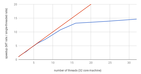
If, on the other other hand, processing time is dominated by your analysis code and not file-reading, then parallelizing the file-reading won’t help. Instead, you want to parallelize your whole analysis, and a good way to do that in Python is with multiprocessing from the Python Standard Library.
If you do split your analysis into multiple processes, you probably don’t want to also parallelize the array-reading within each process. It’s easy to make performance worse by making it too complicated. Particle physics analysis is usually embarrassingly parallel, well suited to splitting the work into independent tasks, each of which is single-threaded.
Another option, of course, is to use a batch system (Condor, Slurm, GRID, etc.). It can be advantageous to parallelize your work across machines with a batch system and across CPU cores with multiprocessing.
TTrees are not the only kinds of objects to analyze in ROOT files; we are also interested in aggregated data in histograms, profiles, and graphs. Uproot uses the ROOT file’s “streamers” to learn how to deserialize any object, but an anonymous deserialization often isn’t useful:
file = uproot3.open("http://scikit-hep.org/uproot3/examples/Event.root")
dict(file.classes())
# {b'ProcessID0;1': uproot3.rootio.TProcessID,
#  b'htime;1': uproot3.rootio.TH1F,
#  b'T;1': uproot3.rootio.TTree,
#  b'hstat;1': uproot3.rootio.TH1F}
processid = file["ProcessID0"]
processid
# <TProcessID b'ProcessID0' at 0x7f36242a3f28>What is a TProcessID?
processid._members()
# ['fName', 'fTitle']
Something with an fName and fTitle…
processid._fName, processid._fTitle     # note the underscore; these are private members
# (b'ProcessID0', b'3ec87674-3aa2-11e9-bb02-0301a8c0beef')
Some C++ classes have Pythonic overloads to make them more useful in Python. Here’s a way to find out which ones have been defined so far:
import pkgutil

[modname for importer, modname, ispkg in pkgutil.walk_packages(uproot3_methods.classes.__path__)]
# ['TGraph',
#  'TGraphAsymmErrors',
#  'TGraphErrors',
#  'TH1',
#  'TH2',
#  'TH3',
#  'THnSparse',
#  'TLorentzVector',
#  'TVector2',
#  'TVector3']
This file contains TH1F objects, which is a subclass of TH1. The TH1 methods will extend it.
file["htime"].edges
# array([ 0.,  1.,  2.,  3.,  4.,  5.,  6.,  7.,  8.,  9., 10.])

file["htime"].values
# array([0.33352208, 0.30402994, 0.32451916, 0.3509729 , 0.36894202,
#        0.30728292, 0.30681205, 0.341563  , 0.16150808, 0.        ],
#       dtype=float32)

file["htime"].show()

#                    0                                                     0.38739
#                    +-----------------------------------------------------------+
# [-inf, 0) 0.021839 |***                                                        |
# [0, 1)    0.33352  |***************************************************        |
# [1, 2)    0.30403  |**********************************************             |
# [2, 3)    0.32452  |*************************************************          |
# [3, 4)    0.35097  |*****************************************************      |
# [4, 5)    0.36894  |********************************************************   |
# [5, 6)    0.30728  |***********************************************            |
# [6, 7)    0.30681  |***********************************************            |
# [7, 8)    0.34156  |****************************************************       |
# [8, 9)    0.16151  |*************************                                  |
# [9, 10)   0        |                                                           |
# [10, inf] 0        |                                                           |
#                    +-----------------------------------------------------------+
The purpose of most of these methods is to extract data, which includes conversion to common Python formats.
uproot3.open("http://scikit-hep.org/uproot3/examples/issue33.root")["cutflow"].show()

#                            0                                               41529
#                            +---------------------------------------------------+
# (underflow)          0     |                                                   |
# Dijet                39551 |*************************************************  |
# MET                  27951 |**********************************                 |
# MuonVeto             27911 |**********************************                 |
# IsoMuonTrackVeto     27861 |**********************************                 |
# ElectronVeto         27737 |**********************************                 |
# IsoElectronTrackVeto 27460 |**********************************                 |
# IsoPionTrackVeto     26751 |*********************************                  |
# (overflow)           0     |                                                   |
# +---------------------------------------------------+file["htime"].pandas()| count | variance | |
|---|---|---|
| Real-Time to write versus time | ||
| [-inf, 0.0) | 0.021839 | 0.000477 |
| [0.0, 1.0) | 0.333522 | 0.111237 |
| [1.0, 2.0) | 0.304030 | 0.092434 |
| [2.0, 3.0) | 0.324519 | 0.105313 |
| [3.0, 4.0) | 0.350973 | 0.123182 |
| [4.0, 5.0) | 0.368942 | 0.136118 |
| [5.0, 6.0) | 0.307283 | 0.094423 |
| [6.0, 7.0) | 0.306812 | 0.094134 |
| [7.0, 8.0) | 0.341563 | 0.116665 |
| [8.0, 9.0) | 0.161508 | 0.026085 |
print(file["htime"].hepdata())

# dependent_variables:
# - header: {name: counts, units: null}
#   qualifiers: []
#   values:
#   - errors:
#     - {label: stat, symerror: 0.33352208137512207}
#     value: 0.33352208137512207
#   - errors:
#     - {label: stat, symerror: 0.3040299415588379}
#     value: 0.3040299415588379
#   - errors:
#     - {label: stat, symerror: 0.32451915740966797}
#     value: 0.32451915740966797
#   - errors:
#     - {label: stat, symerror: 0.35097289085388184}
#     value: 0.35097289085388184
#   - errors:
#     - {label: stat, symerror: 0.3689420223236084}
#     value: 0.3689420223236084
#   - errors:
#     - {label: stat, symerror: 0.3072829246520996}
#     value: 0.3072829246520996
#   - errors:
#     - {label: stat, symerror: 0.306812047958374}
#     value: 0.306812047958374
#   - errors:
#     - {label: stat, symerror: 0.34156298637390137}
#     value: 0.34156298637390137
#   - errors:
#     - {label: stat, symerror: 0.16150808334350586}
#     value: 0.16150808334350586
#   - errors:
#     - {label: stat, symerror: 0.0}
#     value: 0.0
# independent_variables:
# - header: {name: Real-Time to write versus time, units: null}
#   values:
#   - {high: 1.0, low: 0.0}
#   - {high: 2.0, low: 1.0}
#   - {high: 3.0, low: 2.0}
#   - {high: 4.0, low: 3.0}
#   - {high: 5.0, low: 4.0}
#   - {high: 6.0, low: 5.0}
#   - {high: 7.0, low: 6.0}
#   - {high: 8.0, low: 7.0}
#   - {high: 9.0, low: 8.0}
#   - {high: 10.0, low: 9.0}
Numpy histograms, used as a common format through the scientific Python ecosystem, are just a tuple of counts/bin contents and edge positions. (There’s one more edge than contents to cover left and right.)
file["htime"].numpy()
# (array([0.33352208, 0.30402994, 0.32451916, 0.3509729 , 0.36894202,
#         0.30728292, 0.30681205, 0.341563  , 0.16150808, 0.        ],
#        dtype=float32),
#  array([ 0.,  1.,  2.,  3.,  4.,  5.,  6.,  7.,  8.,  9., 10.]))

uproot3.open("http://scikit-hep.org/uproot3/examples/hepdata-example.root")["hpxpy"].numpy()
# (array([[0., 0., 0., ..., 0., 0., 0.],
#         [0., 0., 0., ..., 0., 0., 0.],
#         [0., 0., 0., ..., 0., 0., 0.],
#         ...,
#         [0., 0., 0., ..., 0., 0., 0.],
#         [0., 0., 0., ..., 0., 0., 0.],
#         [0., 0., 0., ..., 0., 0., 0.]], dtype=float32),
#  [(array([-4. , -3.8, -3.6, -3.4, -3.2, -3. , -2.8, -2.6, -2.4, -2.2, -2. ,
#           -1.8, -1.6, -1.4, -1.2, -1. , -0.8, -0.6, -0.4, -0.2,  0. ,  0.2,
#            0.4,  0.6,  0.8,  1. ,  1.2,  1.4,  1.6,  1.8,  2. ,  2.2,  2.4,
#            2.6,  2.8,  3. ,  3.2,  3.4,  3.6,  3.8,  4. ]),
#    array([-4. , -3.8, -3.6, -3.4, -3.2, -3. , -2.8, -2.6, -2.4, -2.2, -2. ,
#           -1.8, -1.6, -1.4, -1.2, -1. , -0.8, -0.6, -0.4, -0.2,  0. ,  0.2,
#            0.4,  0.6,  0.8,  1. ,  1.2,  1.4,  1.6,  1.8,  2. ,  2.2,  2.4,
# 2.6, 2.8, 3. , 3.2, 3.4, 3.6, 3.8, 4. ]))])Uproot has a limited ability to write ROOT files, including TTrees of flat data (non-jagged: single number per event), a variety of histogram types, and TObjString (for metadata).
To write to a ROOT file in Uproot, the file must be opened for writing using uproot3.create, uproot3.recreate, or uproot3.update (corresponding to ROOT’s "CREATE", "RECREATE", and "UPDATE" file modes). The compression level is given by uproot3.ZLIB(n), uproot3.LZMA(n), uproot3.LZ4(n), or None.
file = uproot3.recreate("tmp.root", compression=uproot3.ZLIB(4))Unlike objects created by uproot3.open, you can assign to this file. Just as reading behaves like getting an object from a Python dict, writing behaves like putting an object into a Python dict.
Note: this is a fundamental departure from how ROOT uses names. In ROOT, a name is a part of an object that is also used for lookup. With a dict-like interface, the object need not have a name; only the lookup mechanism (e.g. ROOTDirectory) needs to manage names.
When you write objects to the ROOT file, they can be unnamed things like a Python string, but they get “stamped” with the lookup name once they go into the file.
file["name"] = "Some object, like a TObjString."The object is now in the file. ROOT would be able to open this file and read the data, like this:
We can also read it back in Uproot, like this:
file.keys()
# [b'name;1']

dict(file.classes())
# {b'name;1': uproot3.rootio.TObjString}

file["name"]
# b'Some object, like a TObjString.'
(Notice that it lost its encoding—it is now a bytestring.)
Histograms can be written to the file in the same way: by assignment (choosing a name at the time of assignment). The histograms may be taken from another file and modified,
histogram = uproot3.open("http://scikit-hep.org/uproot3/examples/histograms.root")["one"]
histogram.show()
norm = histogram.allvalues.sum()
for i in range(len(histogram)):
    histogram[i] /= norm
histogram.show()

file["normalized"] = histogram

#                   0                                                       2410.8
#                   +------------------------------------------------------------+
# [-inf, -3)   0    |                                                            |
# [-3, -2.4)   68   |**                                                          |
# [-2.4, -1.8) 285  |*******                                                     |
# [-1.8, -1.2) 755  |*******************                                         |
# [-1.2, -0.6) 1580 |***************************************                     |
# [-0.6, 0)    2296 |*********************************************************   |
# [0, 0.6)     2286 |*********************************************************   |
# [0.6, 1.2)   1570 |***************************************                     |
# [1.2, 1.8)   795  |********************                                        |
# [1.8, 2.4)   289  |*******                                                     |
# [2.4, 3)     76   |**                                                          |
# [3, inf]     0    |                                                            |
#                   +------------------------------------------------------------+
#                     0                                                    0.24108
#                     +----------------------------------------------------------+
# [-inf, -3)   0      |                                                          |
# [-3, -2.4)   0.0068 |**                                                        |
# [-2.4, -1.8) 0.0285 |*******                                                   |
# [-1.8, -1.2) 0.0755 |******************                                        |
# [-1.2, -0.6) 0.158  |**************************************                    |
# [-0.6, 0)    0.2296 |*******************************************************   |
# [0, 0.6)     0.2286 |*******************************************************   |
# [0.6, 1.2)   0.157  |**************************************                    |
# [1.2, 1.8)   0.0795 |*******************                                       |
# [1.8, 2.4)   0.0289 |*******                                                   |
# [2.4, 3)     0.0076 |**                                                        |
# [3, inf]     0      |                                                          |
#                     +----------------------------------------------------------+
or it may be created entirely in Python.
import types
import uproot3_methods.classes.TH1

class MyTH1(uproot3_methods.classes.TH1.Methods, list):
    def __init__(self, low, high, values, title=""):
        self._fXaxis = types.SimpleNamespace()
        self._fXaxis._fNbins = len(values)
        self._fXaxis._fXmin = low
        self._fXaxis._fXmax = high
        for x in values:
            self.append(float(x))
        self._fTitle = title
        self._classname = "TH1F"

histogram = MyTH1(-5, 5, [0, 1, 1, 1, 1, 1, 1, 1, 1, 1, 1, 0])

file["synthetic"] = histogram
file["synthetic"].show()
# 0 1.05
# +--------------------------------------------------------+
# [-inf, -5) 0 | |
# [-5, -4.1667) 1 |***************************************************** |
# [-4.1667, -3.3333) 1 |***************************************************** |
# [-3.3333, -2.5) 1 |***************************************************** |
# [-2.5, -1.6667) 1 |***************************************************** |
# [-1.6667, -0.83333) 1 |***************************************************** |
# [-0.83333, 0) 1 |***************************************************** |
# [0, 0.83333) 1 |***************************************************** |
# [0.83333, 1.6667) 1 |***************************************************** |
# [1.6667, 2.5) 1 |***************************************************** |
# [2.5, 3.3333) 1 |***************************************************** |
# [5, inf] 0 | |
# +--------------------------------------------------------+But it is particularly useful that Uproot recognizes Numpy histograms, which may have come from other libraries.
file["from_numpy"] = numpy.histogram(numpy.random.normal(0, 1, 10000))file["from_numpy"].show()
# 0 2993.6
# +-----------------------------------------------------+
# [-inf, -3.6179) 0 | |
# [-3.6179, -2.8738) 22 | |
# [-2.8738, -2.1296) 127 |** |
# [-2.1296, -1.3854) 632 |*********** |
# [-1.3854, -0.64124) 1814 |******************************** |
# [-0.64124, 0.10294) 2851 |************************************************** |
# [0.10294, 0.84711) 2602 |********************************************** |
# [0.84711, 1.5913) 1391 |************************* |
# [1.5913, 2.3355) 464 |******** |
# [2.3355, 3.0796) 85 |** |
# [3.0796, 3.8238) 12 | |
# [3.8238, inf] 0 | |
# +-----------------------------------------------------+file["from_numpy2d"] = numpy.histogram2d(numpy.random.normal(0, 1, 10000),
numpy.random.normal(0, 1, 10000))file["from_numpy2d"].numpy()
# (array([[ 0., 0., 0., 0., 1., 4., 2., 0., 0., 0.],
# [ 0., 2., 4., 10., 15., 17., 9., 3., 1., 0.],
# [ 0., 3., 14., 50., 90., 86., 58., 23., 4., 1.],
# [ 2., 10., 53., 174., 348., 337., 239., 68., 12., 0.],
# [ 2., 26., 136., 367., 675., 740., 461., 141., 32., 5.],
# [ 4., 19., 146., 466., 790., 873., 503., 154., 30., 4.],
# [ 1., 20., 91., 294., 515., 531., 299., 132., 21., 2.],
# [ 0., 2., 32., 109., 195., 193., 131., 42., 5., 0.],
# [ 1., 2., 8., 22., 42., 42., 25., 9., 2., 0.],
# [ 0., 0., 0., 3., 8., 2., 5., 0., 0., 0.]]),
# [(array([-4.06785591, -3.29187021, -2.51588451, -1.7398988 , -0.9639131 ,
# -0.1879274 , 0.5880583 , 1.36404401, 2.14002971, 2.91601541,
# 3.69200111]),
# array([-3.87804614, -3.1115391 , -2.34503205, -1.578525 , -0.81201795,
# -0.0455109 , 0.72099614, 1.48750319, 2.25401024, 3.02051729,
# 3.78702434]))])As of now, Uproot can write TTrees whose branches are basic types (integers and floating-point numbers).
Basic usage:
import uproot3
import numpy

with uproot3.recreate("example.root") as f:
    f["t"] = uproot3.newtree({"branch": "int32"})
    f["t"].extend({"branch": numpy.array([1, 2, 3, 4, 5])})
You can specify the branches in your TTree explicitly:
t = uproot3.newtree({"branch1": int,
                     "branch2": numpy.int32,
                     "branch3": uproot3.newbranch(numpy.float64, title="This is the title")})
uproot3.newtree() takes a Python dictionary as an argument, where the key is the name of the branch and the value is the branch object or type of branch.
We can specify the title, the flushsize and the compression while creating the tree.
This is an example of how you would add a title to your tree:
tree = uproot3.newtree(branchdict, title="TTree Title")To specify the title of the branch, similar to how you would add a title to a tree:
b = uproot3.newbranch("int32", title="This is the title")branch1
branch2
The suggested interface of writing baskets to the TTree is using the extend method:
f["t"].extend({"branch1": numpy.array([1, 2, 3, 4, 5]), "branch2": [6, 7, 8, 9, 10]})Remember to add entries to all the branches and the number of entries added to the branches is the same!
What must be kept in mind is that if you write a lot of small baskets, it is going to be much less performant(slow and will increase the size of the file) than writing large arrays into the TTree as a single basket -> Uproot's implementation is optimized for large array oriented operations.
Low level interface
If you want, you can write a basket to only 1 branch. But remember to add equal number of baskets to the other branches as well as ROOT assumes that all the branches have equal number of baskets and will not read the non-uniform baskets.
f["t"]["branch1"].newbasket([1, 2, 3])Add 3 more basket data to branch2!
f["t"]["branch2"].newbasket([91, 92, 93])By default, the baskets of all the branches are compressed depending on the compression set for the file.
You can specify the compression of all the branches if you want it to be separate from the compression specified for the entire file by using the uproot3.newtree() method.
You can also specify the compression of each branch individually by using the uproot3.newbranch() method.
b1 = uproot3.newbranch("i4", compression=uproot3.ZLIB(5))
b2 = uproot3.newbranch("i8", compression=uproot3.LZMA(4))
b3 = uproot3.newbranch("f4")

branchdict = {"branch1": b1, "branch2": b2, "branch3": b3}
tree = uproot3.newtree(branchdict, compression=uproot3.LZ4(4))
with uproot3.recreate("example.root", compression=uproot3.LZMA(5)) as f:
    f["t"] = tree
f["t"].extend({"branch1": [1]*1000, "branch2": [2]*1000, "branch3": [3]*1000})Support for this work was provided by NSF cooperative agreement OAC-1836650 (IRIS-HEP), grant OAC-1450377 (DIANA/HEP) and PHY-1520942 (US-CMS LHC Ops).
Thanks especially to the gracious help of Uproot contributors!