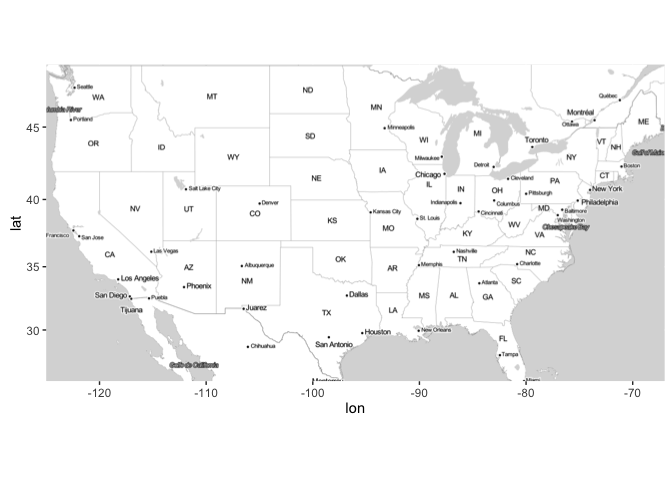
ggmap makes it easy to retrieve raster map tiles from popular online mapping services like Google Maps, OpenStreetMap, Stamen Maps, and plot them using the ggplot2 framework:
library(ggmap)

us <- c(left = -125, bottom = 25.75, right = -67, top = 49)
map <- get_stamenmap(us, zoom = 5, maptype = "toner-lite")
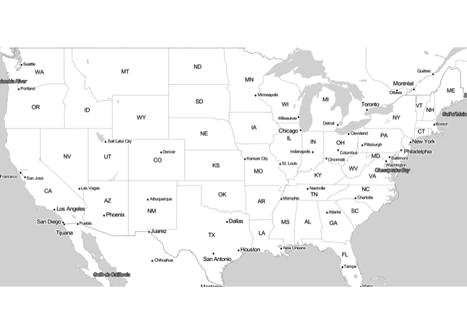
ggmap(map)ggmap(map, extent = "device")Use qmplot() in the same way you'd use qplot(), but with a map automatically added in the background:
library(dplyr)

# only violent crimes
violent_crimes <- filter(crime,
  offense != "auto theft", offense != "theft", offense != "burglary"
)

# rank violent crimes
violent_crimes$offense <- factor(
  violent_crimes$offense,
  levels = c("robbery", "aggravated assault", "rape", "murder")
)

# restrict to downtown
violent_crimes <- filter(violent_crimes,
  -95.39681 <= lon & lon <= -95.34188,
   29.73631 <= lat & lat <=  29.78400
)

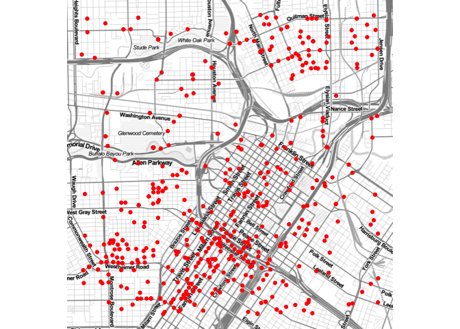
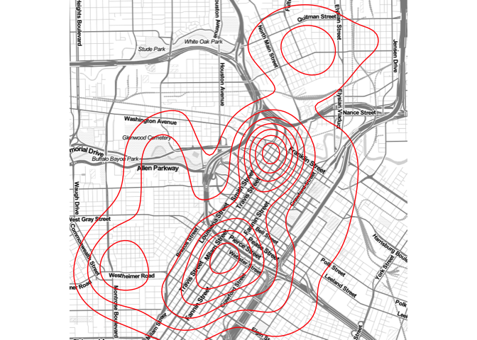
qmplot(lon, lat, data = violent_crimes, maptype = "toner-lite", color = I("red"))qmplot(lon, lat, data = violent_crimes, maptype = "toner-lite", geom = "density2d", color = I("red"))Since ggmap's built on top of ggplot2, all your usual ggplot2 stuff (geoms, polishing, etc.) will work, and there are some unique graphing perks ggmap brings to the table, too.
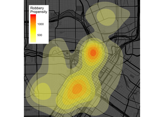
robberies <- violent_crimes %>% filter(offense == "robbery")

qmplot(lon, lat, data = violent_crimes, geom = "blank", zoom = 15, maptype = "toner-background", darken = .7, legend = "topleft") +
  stat_density_2d(aes(fill = ..level..), geom = "polygon", alpha = .3, color = NA) +
  scale_fill_gradient2("Robbery\nPropensity", low = "white", mid = "yellow", high = "red", midpoint = 650)
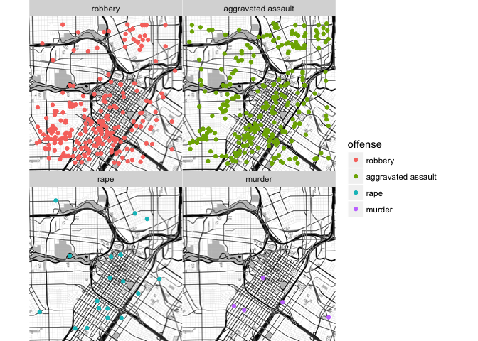
Faceting works, too:
qmplot(lon, lat, data = violent_crimes, maptype = "toner-background", color = offense) +
  facet_wrap(~ offense)
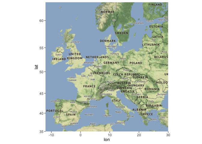
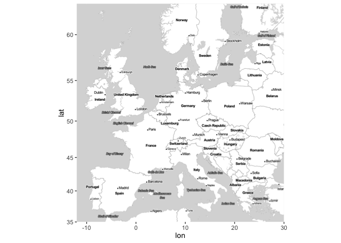
For convenience, here's a map of Europe:
europe <- c(left = -12, bottom = 35, right = 30, top = 63)
get_stamenmap(europe, zoom = 5) %>% ggmap()get_stamenmap(europe, zoom = 5, maptype = "toner-lite") %>% ggmap()Google Maps can be used just as easily. However, since Google Maps use a center/zoom specification, their input is a bit different:
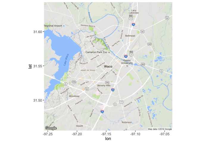
get_googlemap("waco texas", zoom = 12) %>% ggmap()
#  Source : https://maps.googleapis.com/maps/api/staticmap?center=waco+texas&zoom=12&size=640x640&scale=2&maptype=terrain
#  Source : https://maps.googleapis.com/maps/api/geocode/json?address=waco%20texas
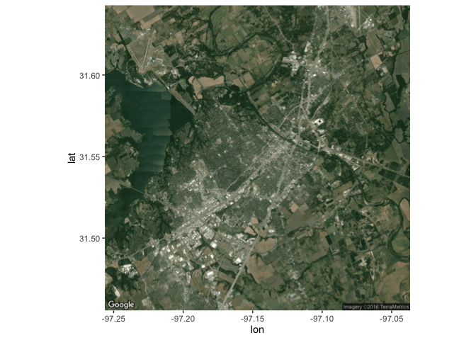
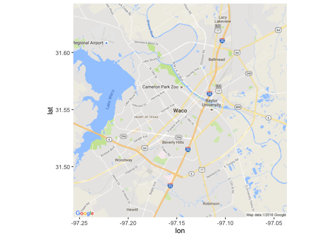
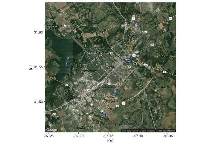
Moreover, you can get various different styles of Google Maps with ggmap (just like Stamen Maps):
get_googlemap("waco texas", zoom = 12, maptype = "satellite") %>% ggmap()
#  Source : https://maps.googleapis.com/maps/api/staticmap?center=waco+texas&zoom=12&size=640x640&scale=2&maptype=satellite
# Source : https://maps.googleapis.com/maps/api/geocode/json?address=waco%20texasget_googlemap("waco texas", zoom = 12, maptype = "roadmap") %>% ggmap()
# Source : https://maps.googleapis.com/maps/api/staticmap?center=waco+texas&zoom=12&size=640x640&scale=2&maptype=roadmap
# Source : https://maps.googleapis.com/maps/api/geocode/json?address=waco%20texasget_googlemap("waco texas", zoom = 12, maptype = "hybrid") %>% ggmap()
# Source : https://maps.googleapis.com/maps/api/staticmap?center=waco+texas&zoom=12&size=640x640&scale=2&maptype=hybrid
# Source : https://maps.googleapis.com/maps/api/geocode/json?address=waco%20texasGoogle's geocoding and reverse geocoding API's are available through geocode() and revgeocode(), respectively:
geocode("1301 S University Parks Dr, Waco, TX 76798")
#  Source : https://maps.googleapis.com/maps/api/geocode/json?address=1301%20S%20University%20Parks%20Dr%2C%20Waco%2C%20TX%2076798
#         lon      lat
#  1 -97.1161 31.55098
revgeocode(c(lon = -97.1161, lat = 31.55098))
#  Information from URL : https://maps.googleapis.com/maps/api/geocode/json?latlng=31.55098,-97.1161
#  [1] "1301 S University Parks Dr, Waco, TX 76706, USA"
There is also a mutate_geocode() that works similarly to dplyr's mutate() function:
library(tidyverse)
#  Loading tidyverse: tibble
#  Loading tidyverse: tidyr
#  Loading tidyverse: readr
#  Loading tidyverse: purrr
#  Conflicts with tidy packages ----------------------------------------------
#  filter(): dplyr, stats
#  lag():    dplyr, stats
tb <- data_frame(address = c("1600 Pennsylvania Avenue, Washington DC", "", "waco texas"))
tb %>% mutate_geocode(address)
#  Source : https://maps.googleapis.com/maps/api/geocode/json?address=1600%20Pennsylvania%20Avenue%2C%20Washington%20DC
#  Source : https://maps.googleapis.com/maps/api/geocode/json?address=waco%20texas
#  # A tibble: 3 × 3
#                                    address       lon      lat
#                                      <chr>     <dbl>    <dbl>
#  1 1600 Pennsylvania Avenue, Washington DC -76.98184 38.87920
#  2                                                NA       NA
#  3                              waco texas -97.14667 31.54933
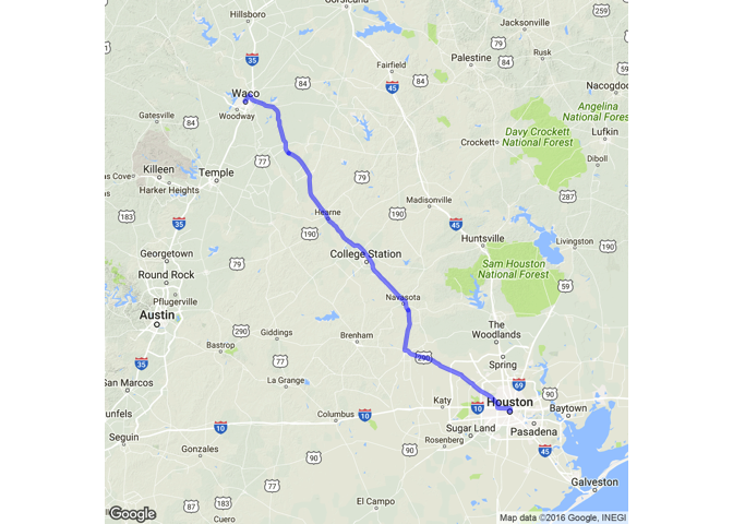
Treks use Google's routing API to give you routes (route() and trek() give slightly different results; the latter hugs roads):
trek_df <- trek("houson, texas", "waco, texas", structure = "route")
#  Source : https://maps.googleapis.com/maps/api/directions/json?origin=houson%2C%20texas&destination=waco%2C%20texas&mode=driving&units=metric&alternatives=false
qmap("college station, texas", zoom = 8) +
  geom_path(
    aes(x = lon, y = lat),  colour = "blue",
    size = 1.5, alpha = .5,
    data = trek_df, lineend = "round"
  )
#  Source : https://maps.googleapis.com/maps/api/staticmap?center=college+station,+texas&zoom=8&size=640x640&scale=2&maptype=terrain&language=en-EN
#  Source : https://maps.googleapis.com/maps/api/geocode/json?address=college%20station%2C%20texas
(They also provide information on how long it takes to get from point A to point B.)
Map distances, in both length and anticipated time, can be computed with mapdist()). Moreover the function is vectorized:
mapdist(c("houston, texas", "dallas"), "waco, texas")
#  Source : https://maps.googleapis.com/maps/api/distancematrix/json?origins=dallas&destinations=waco%2C%20texas&mode=driving&language=en-EN
#  Source : https://maps.googleapis.com/maps/api/distancematrix/json?origins=houston%2C%20texas&destinations=waco%2C%20texas&mode=driving&language=en-EN
#              from          to      m      km     miles seconds   minutes
#  1 houston, texas waco, texas 298242 298.242 185.32758   10176 169.60000
#  2         dallas waco, texas 152652 152.652  94.85795    5291  88.18333
#       hours
#  1 2.826667
# 2 1.469722If you have a Google API key, you can exceed the standard limits Google places on queries. By default, when ggmap is loaded it will set the following credentials and limits:
ggmap_credentials()
#  Google -
#     key :
#     account_type : standard
#     day_limit : 2500
#     second_limit : 50
#     client :
#     signature :
Look at the documentation of ?register_google() to learn more. If you do have an API key, you set it with:
register_google(key = "[your key here]", account_type = "premium", day_limit = 100000)
ggmap_credentials()
#  Google -
#     key : [your key here]
#     account_type : premium
#     day_limit : 1e+05
#     second_limit : 50
#     client :
#     signature :
These will then be used and checked when creating the query URL:
register_google(key = "AbCdEfGhIjKlMnOpQrStUvWxYz")
get_googlemap("waco texas", urlonly = TRUE)
#  [1] "https://maps.googleapis.com/maps/api/staticmap?center=waco+texas&zoom=10&size=640x640&scale=2&maptype=terrain&key=AbCdEfGhIjKlMnOpQrStUvWxYz"
For anything that hasn't been implemente (URL-wise), you can inject code into the query usin g inject:
get_googlemap("waco texas", urlonly = TRUE, inject = "otherItem = Stuff")
# [1] "https://maps.googleapis.com/maps/api/staticmap?center=waco+texas&zoom=10&size=640x640&scale=2&maptype=terrain&key=AbCdEfGhIjKlMnOpQrStUvWxYz&otherItem%20=%20Stuff"-
From CRAN:
install.packages("ggmap") -
From Github:
devtools::install_github("dkahle/ggmap")
