Generalizing Convolutional Neural Networks for Equivariance to Lie Groups on Arbitrary Continuous Data

This repo contains the implementation and the experiments for the paper

Generalizing Convolutional Neural Networks for Equivariance to Lie Groups on Aribitrary Continuous Data

by Marc Finzi, Samuel Stanton, Pavel Izmailov, and Andrew Gordon Wilson.

If you find our work helpful, please cite it with

@article{finzi2020generalizing,
  title={Generalizing Convolutional Neural Networks for Equivariance to Lie Groups on Arbitrary Continuous Data},
  author={Finzi, Marc and Stanton, Samuel and Izmailov, Pavel and Wilson, Andrew Gordon},
  journal={arXiv preprint arXiv:2002.12880},
  year={2020}
}

Introduction

LieConv is an equivariant convolutional layer that can be applied on generic coordinate-value data and instantiated with the symmetries of a given Lie Group. LieConv was designed with rapid prototyping in mind, we believe that researchers and engineers should be able to experiment with multiple symmetry groups rather than being locked into using a given symmetry by the method.

Installation

To install as a package, run pip install git+https://github.com/mfinzi/LieConv#egg=LieConv. Dependencies will be checked and installed from the setup.py file.

To run the scripts you will need to clone the repo and install it locally. You can use the commands below.

git clone https://github.com/mfinzi/LieConv.git
cd LieConv
pip install -e .

For the optional graphnets and tensorboardX functionality you can replace the last line with pip install -e .[GN,TBX]

Dependencies

Dependencies will be automatically installed from the setup.py file with pip install -e . but they are listed here for reference.

Python 3.7+
PyTorch 1.3.0+
torchvision
olive-oil-ml
torchdiffeq
(optional) [torch-scatter,torch-sparse,torch-cluster,torch-geometric]
(optional) tensorboardX

Architecture

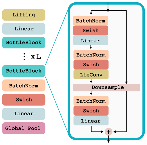
For all experiments, we use the same LieResNet architecture where LieConv replaces an ordinary convolutional layer. This network can act on inputs that are any collection of coordinates and values {x_i,v_i}_{i=1}^N, and is detailed below and implemented in lie_conv.lieconv. We apply this same network architecture to RotMNIST dataset, the QM9 molecular property prediction dataset, and to the modeling of Hamiltonian dynamical systems. The architecture is shown below.

RotMNIST Experiments

We provide commands to run LieConv on the RotMNIST data for different groups. The commands share hyper-parameters except for the name of the group and the --alpha parameter that trades off between group and orbit distance in the neighborhoods. Aug specifies whether to use SO(2) data augmentation.

# Trivial
python examples/train_img.py --num_epochs=500 --trainer_config "{'log_suffix':'mnistTrivial'}" \
  --net_config "{'k':128,'total_ds':.1,'fill':.1,'nbhd':25,'group':Trivial(2)}" \
  --bs 25 --lr .003 --split "{'train':12000}" --aug=True

# T2
python examples/train_img.py --num_epochs=500 --trainer_config "{'log_suffix':'mnistT2'}" \
   --net_config "{'k':128,'total_ds':.1,'fill':.1,'nbhd':25,'group':T(2)}" \
   --bs 25 --lr .003 --split "{'train':12000}" --aug=True

# SO2
python examples/train_img.py --num_epochs=500 --trainer_config "{'log_suffix':'mnistSO2'}" \
  --net_config "{'k':128,'total_ds':.1,'fill':.1,'nbhd':25,'group':SO2(.2)}" \
  --bs 25 --lr .003 --split "{'train':12000}" --aug=True

#RxSO2
python examples/train_img.py --num_epochs=500 --trainer_config "{'log_suffix':'mnistRxSO2'}" \
  --net_config "{'k':128,'total_ds':.1,'fill':.1,'nbhd':25,'group':RxSO2(.3)}" \
  --bs 25 --lr 3e-3 --split "{'train':12000}" --aug=True

#SE2
python examples/train_img.py --num_epochs=500 --trainer_config "{'log_suffix':'mnistSE2'}" \
  --net_config "{'k':128,'total_ds':.1,'fill':.1,'nbhd':25,'group':SE2(.05),'liftsamples':2}" \
  --bs 25 --lr 3e-3 --split "{'train':12000}" --aug=True

Using the commands above we obtain the following test errors (%) for the different groups:

Trivial	Tx	T2	SO2	RxSO2	SE2
1.44	1.35	1.32	1.27	1.13	1.13

For the curious minded, we have added 3 additional groups: Translation in x only:Tx(2), and Translation in y only:Ty(2), and scaling Scaling:Rx(.1)

QM9 Molecular Experiments

To train the model on QM9 molecular property regression, run the script below with the --task specified by the strings from the first row of the following table. The table shows Test MAE for each of the tasks with the T(3) group trained for 500 epochs which takes ~24 hrs on a single 1080Ti GPU. The --aug command specifies whether to use SO(3) data augmentation.

# T(3)
python examples/train_molec.py --task 'homo' --lr 3e-3 --aug True --num_epochs 500 --num_layers 6 \
  --log_suffix 't3_run_name' --network MolecLieResNet --save=True \
  --net_config "{'group':T(3),'fill':1.}"

# SE3
python examples/train_molec.py --task 'homo' --lr 3e-3 --aug True --num_epochs 500 --num_layers 6 \
--log_suffix 'se3_run_name' --network MolecLieResNet --recenter=True --bs 75 --save=True \
--net_config "{'group':SE3(.2),'fill':1/2,'liftsamples':4, 'nbhd':25}"

# Trivial(3)
python examples/train_molec.py --task 'homo' --lr 3e-3 --aug True --num_epochs 500 --num_layers 6 \
  --log_suffix 'trivial_run_name' --network MolecLieResNet --save=True \
  --net_config "{'group':Trivial(3),'fill':1.}"

# SO3
python examples/train_molec.py --task 'homo' --lr 3e-3 --aug True --num_epochs 500 --num_layers 6 \
  --log_suffix 'so3_run_name' --network MolecLieResNet  --recenter=True --bs 75 --save=True \
  --net_config "{'group':SO3(.2),'fill':1/2,'liftsamples':4, 'nbhd':25}"

	Task	alpha	gap	homo	lumo	mu	Cv	G	H	r2	U	U0	zpve
Group	Units	bohr^3	meV	meV	meV	Debye	cal/mol K	meV	meV	bohr^2	meV	meV	meV
T(3)	MAE	.084	49	30	25	.032	.038	22	24	.800	19	19	2.280

Group Comparisons on HOMO task

Trivial	SO(3)	T(3)	SE(3)
31.7	65.4	29.4	26.8

Spring Dynamics Experiments

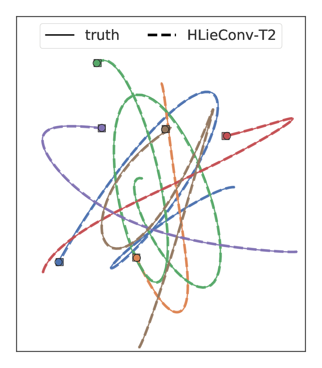
We apply our method in the modeling of a multi particle spring system, an example of a Hamiltonian system that conserves linear and angular momentum. To train using the HLieResNet model, simply run

python examples/train_springs.py --num_epochs 100 --n_train 3000 \
  --network HLieResNet --net_cfg "{'group':T(2),'k':384,'num_layers':4}" --lr 1e-3

where Trivial(2), T(2), SO2() can be substituted in for T(2) to specify the group equivariance. The first time this command is run will take a while as the dataset is generated and then saved to disk.

The FC, HFC, OGN, and HOGN baselines can be run as follows:

python examples/train_springs.py --num_epochs 100 --n_train 3000 \
  --network FC --net_cfg "{'k':256,'num_layers':4}" --lr 1e-2

python examples/train_springs.py --num_epochs 100 --n_train 3000 \
  --network HFC --net_cfg "{'k':256,'num_layers':4}" --lr 1e-2

python examples/train_springs.py --num_epochs 100 --n_train 3000 \
  --network OGN --net_cfg "{'k':256}" --lr 1e-2

python examples/train_springs.py --num_epochs 100 --n_train 3000 \
  --network HOGN --net_cfg "{'k':256}" --lr 1e-2

Note that OGN and HOGN require the graphnet functionality to be installed with pip install -e .[GN].

In the Figure below we show the predictions of LieConv and HOGN, a SOTA architecture for modeling physical systems, on a 6-body spring dynamics problem.

mfinzi / LieConv