Advanced Lane Finding
In this project, the idea is to improve the approach in Lane Line Finding with new techniques learned from the Self-Driving car Engineer Nanodegree from Udacity.
You can find a result video here
Table of contents
Camera calibration
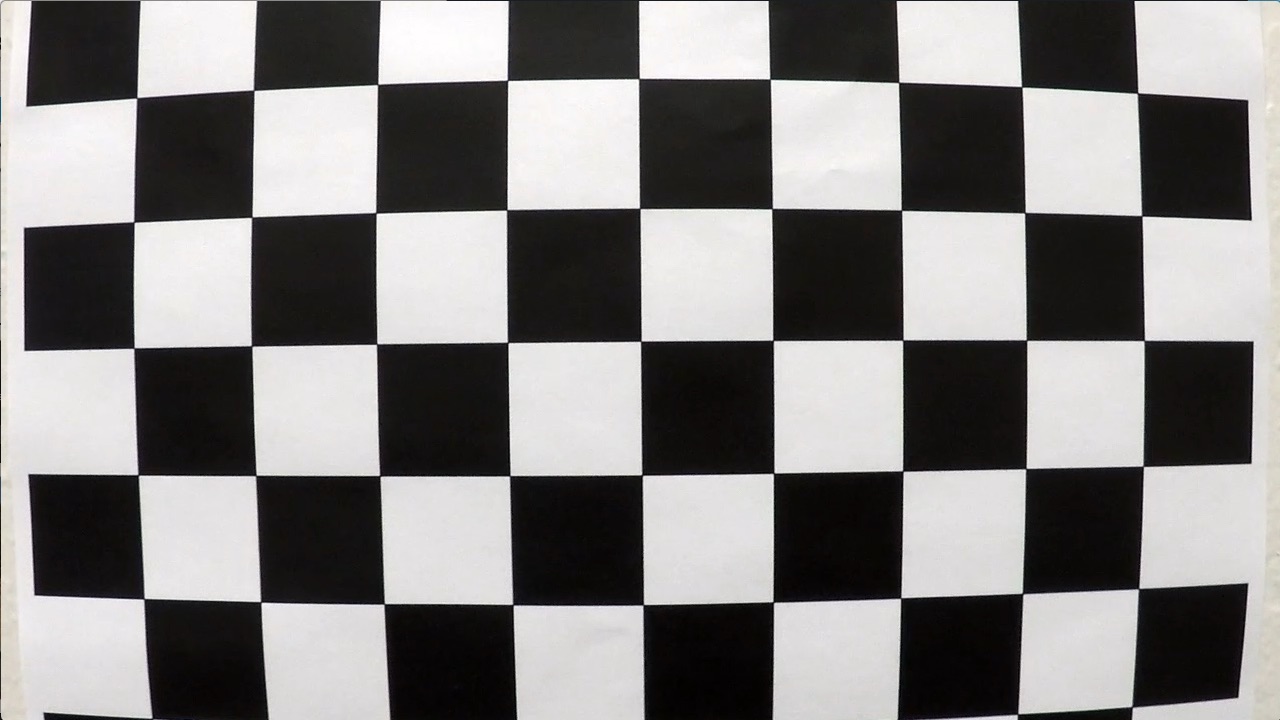
The first and very important step in our image processing pipeline is camera calibration. This is a step sometimes neglected, but very important to have consistent and correct images. Cameras are made with lenses, and because they do not represent a perfect pinhole model, their lenses distort the formed image. However, using camera calibration, we can evaluate this distortion and apply an undistortion to the image.
One of the ways to calibrate a camera is to prepare a chessboard pattern and take multiple pictures of it, in many
different angles and positions. You can find these pictures in folder camera_cal. Then assuming (x,y,z) coordinates
for the chessboard corners and that it is fixed on plane where z=0, we use we use cv2.findChessboardCorners
to find the correspondent corners in the image and cv2.calibrateCamera to match camera
to find the chessboard pattern in the multiple images provided. With this chessboard pattern detected, we then
use cv2.calibrateCamera to find the camera calibration parameters. For a detailed explanation on how
camera calibration works in Python, please follow this tutorial.
Generally, you don't have to calibrate your camera all the time. Preferably, you will do it once, then store the parameters. Given that, I've separated the camera calibration in a separate script. You can run it using
python3 camera_calibration.py
This script will store a calibration.p file with the calibration parameters.
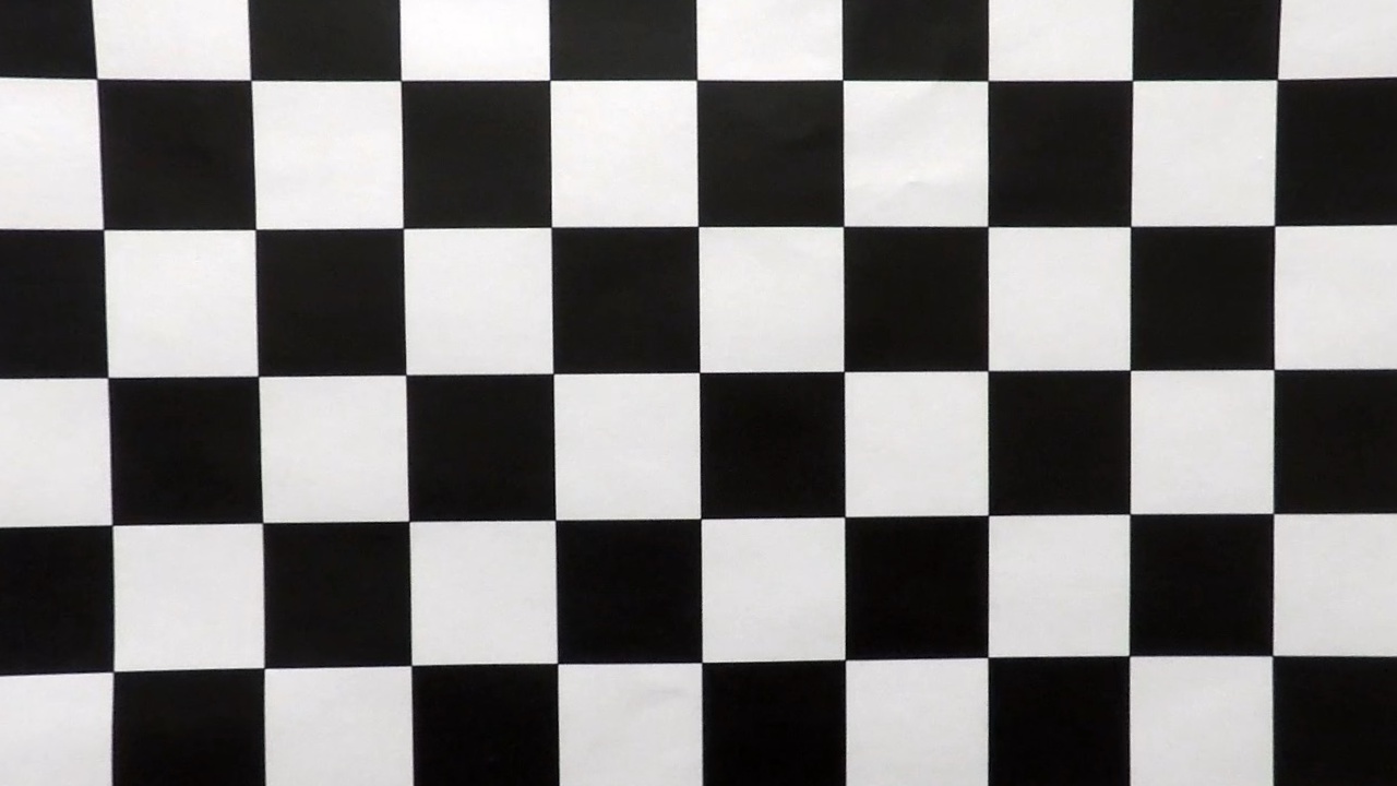
With the camera calibration parameters on hand, now we should undistort the image. For that, we can
reload the parameters from calibration.p, then use cv2.undistort to get the image.
Image processing pipeline
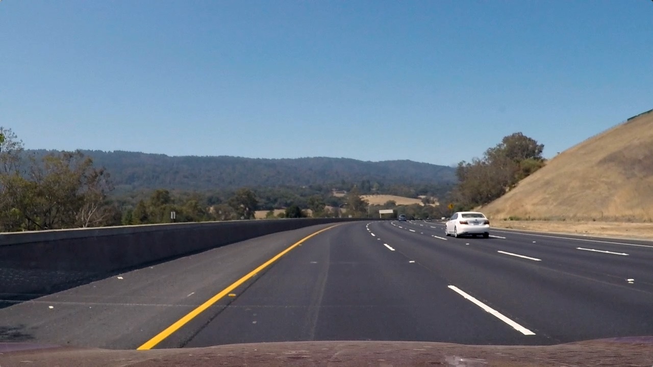
Now, we will go through each step ran at every frame of the video. We start with this example image:
Thresholded binary image
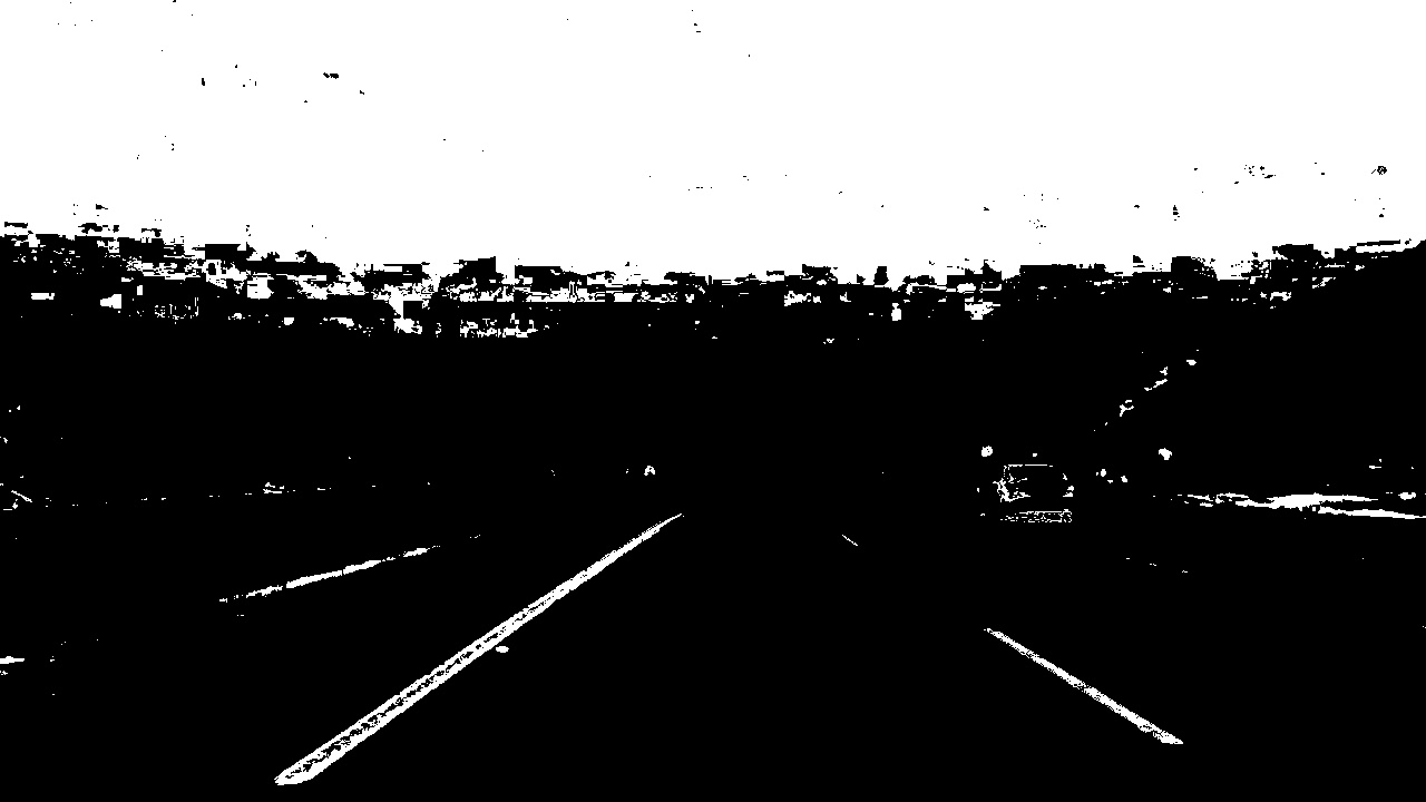
After undistorting the image, we then proceed to create a binary thresholded image. In this step, we transform the video frame into a binary image (either white or black). We do so in order to get an easier to treat image for the following steps. The first step is to calculate the HSL representation of the image. HSL (hue, saturation and lightness) is another way to represent color spaces, other than RBG. We use the S channel because it is immune to lightness and color variations in the image. This is the output of the S channel binary image:
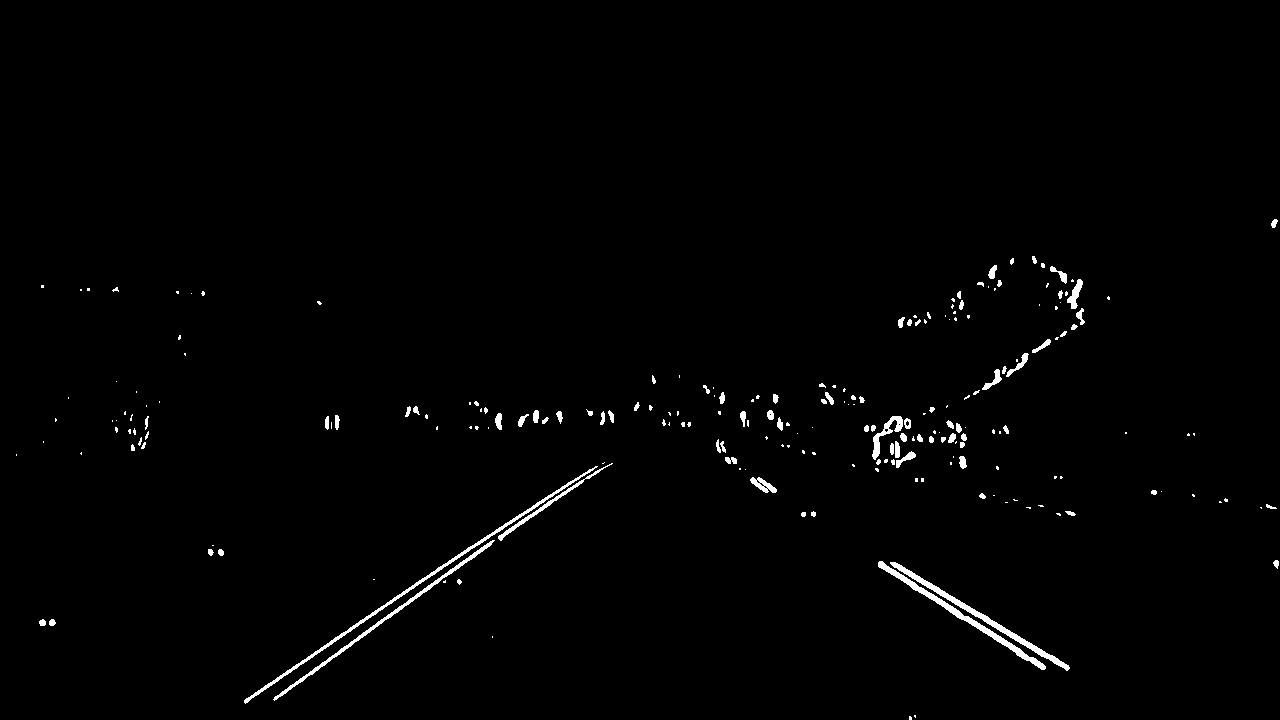
Then, we use the L channel to calculate the Sobel-Feldman Operator. The Sobel operator is a joint of a Gaussian smoothing and a Canny transform of the image. Differently from Canny transform, the Sobel operator can have a derivative direction, so we can consider derivatives in a specific orientation. This is the output of the binary Sobel transform on L channel:
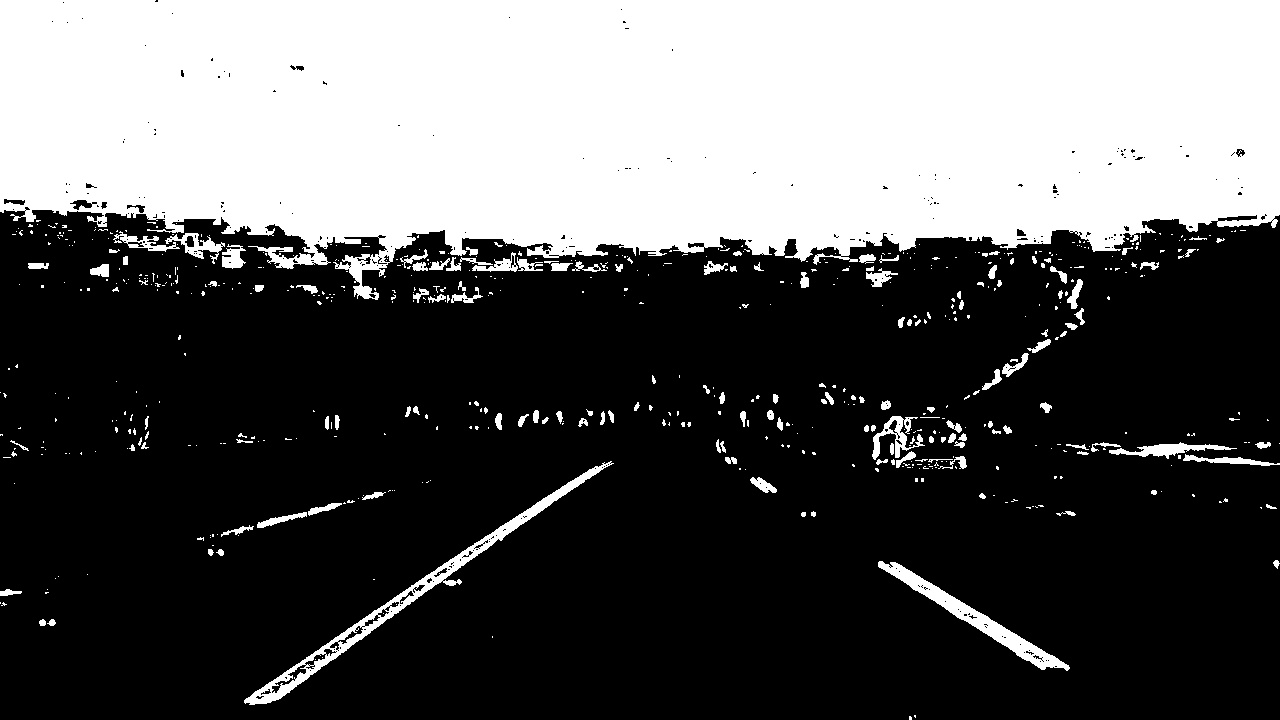
Combining both with a AND operator, we get our final thresholded binary image:
Where lanes are more defined on this final image than on each of them separately.
The code can be found on thresholding.py
Perspective transform
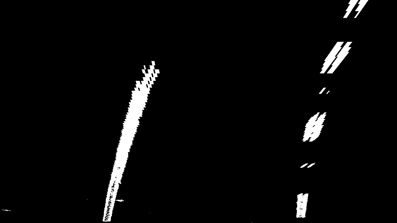
After getting the binary images, we then perform a perspective transform to the image, so we can get a birds-eye view of the lanes. This will be useful for detecting the lane curvatures on the next step. For performing the perspective transform, I assumed that the camera is centered on the vehicle and I applied a transform which transformed the trapezoid formed by the lanes on the image into destination points on the transformed image:
trapezoid: [[200, 720], [590, 450], [690, 450], [1130, 720]]
dest_points: [[320, 720], [320, 0], [960, 0], [960, 720]]
This gives the following result on the binary image:
The code can be found on perspective.py
Detecting lane pixels
I used a sliding window technique to find where most pixels on each vertical window is, and thus, determinate the position of the lane. Then, I fitted these positions to a second-order polynomial. I also keep the polynomial parameters of the last 30 fitted polynomials and use the average to display the information to the user. This greatly improved algorithm stability and display clarity.
The code can be found on src/lane_polyfit.py
Warping to the original image
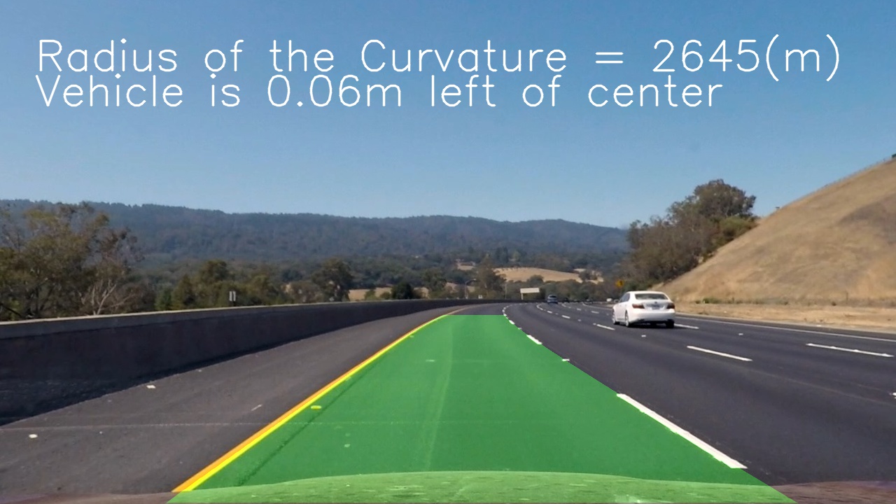
I created a solid with the polynomial curves of the evaluated parameters of the current average of the polynomial parameters. The result looks like this:
The code can be found on lane_polyfit.py
Parameters
All the parameters of the code are configurable through config.yaml file. I have implemented a python module that takes care of the parameters and reads the yaml file when user requests for it.
Try it yourself
First of all, please follow the instructions here to set up your conda environment. Then, on your terminal use:
conda activate carnd-term1Then, run the camera_calibration.py
python3 camera_calibration.pyIt will produce the file calibration.p. Then, to get video output, you can run:
python3 project_video.pyIt will process the video and put it on folder output_videos.
If you want to have the output of each image processing step, you can run:
python3 test_images_lane_lines.pyIt will output the images of each step of the pipeline on folder output_images.
Possible improvements
One of the ways we could improve is to use other color space transformations and explore which ones could also be suitable for detecting lane lines. Also, the code makes an assumption of centimeters per pixel scale when calculating the radius of curvature and position on lane. We could find other ways (with laser scan sensors for example) to measure this value directly and avoid this approximation.
