- overall for neural network and deep learning.
- interview to Geoffrey Hinton
- Python basic
- Avoid use for-loop or while loop in computation to some extend. Try best to make matrix computation.
- Using numpy function to complete matrix/vector computation.
- Matrix/vector operated by numeric would be "broadcasting"
- 0-layer logistic regression(only a activation node)
- if just make a simple logistic regression, w and b can be initialized in "zero" vector. But for multi-layer neural network w can't be initialized as "zero". The reason would be introduced in next section.
- Different learning rate would influence performance deeply.
- Implement a simple 1-layer NN
- Compared with previous logistic regression, 1-layer NN can solve some non-linear separable problem.
- W must be initialized by a random normal. It is because that assigning different weights to each node in hidden layer can trigger them to learn different decision boundary. If initializing zero or same weight to each weight, it would result to a balance where each node learns same decision boundary, and then the whole network would be same with only on node. But, b can be initialized as "zero". Zero is related with training data.
- The loss function is chosen as cross-entropy for logistic activation. Here, the square loss + logistic would become as a non-convex which has many local minima.
- Cost function = averaging(loss function). Cost function would involve in back-propagation.
- Learning rate, hidden layer size and number of nodes are hyper-parameter. Kinds of method can be used to choose them. Try them by your self.
-
Deep neural network: step by step
- The difference from shallow neural network is just using loop to finish forward and back propagation.
- Cultivate yourself for a good writing habit.
- Superscript
$[l]$ denotes a quantity associated with the$l^{th}$ layer. Example:$a^{[L]}$ is the$L^{th}$ layer activation.$W^{[L]}$ and$b^{[L]}$ are the$L^{th}$ layer parameters. - Superscript
$(i)$ denotes a quantity associated with the$i^{th}$ example. Example:$x^{(i)}$ is the$i^{th}$ training example. - Lower-script
$i$ denotes the$i^{th}$ entry of a vector. Example:$a^{[l]}_i$ denotes the$i^{th}$ entry of the$l^{th}$ layer's activations).
- Superscript
-
Activation function choose: - Logistic regression: Just for last layer for binary classification. Almost no ones choose it as activation function in hidden lay. - Tanh: better than logistic because the median point locates in right zero, but logistic locates in 0.5. - Relu: most used in current days. High speed even it is not differential, but still works well. - Leaky relu: just a transform for relu when w less than zero, multiply a small number to w.
Don't be lazy and do by yourself.
- Initialization
- Zeros initialization
- As said before, the symmetry can't be broken. all of nodes would be trained in same weight. Performance of it would very poor around 50%. The cost wouldn't get changed as long as iteration.
- Random initialization
- the parameters are initialized from normal distribution . The result would get better. After generate an array of parameter, it is better to multiply a small number like 0.01 to make parameter approach to zero.
- Xavier initialization:
- A substitute of small number is to scale it by layer size.
- Sigmoid/Tanh: sqrt(1./layers_dims[l-1])
- Relu: sqrt(2./layers_dims[l-1])
- A substitute of small number is to scale it by layer size.
- Don't initialize to values that are too large.
- Zeros initialization
- Regularization
- L2-regularization
- In cost function, add a item to the cost computation behind of the equation cost = cross_entropy_cost + L2_regularization_cost
- In back_propogation, add a item to each layer of dw as W*lambd/m.
- Increase the value of lambd would decrease the value of weight and reduce over-fitting of model.
- Dropout
- Normal dropout: In training phase, use dropout to randomly choose neutrons in hidden layers. In test phase, scale activation to original ones by multiplying dropout rate p.
- Inverted dropout(common used): also use dropout proportion of hidden units, then divide by 1/p to restore the scale of units for next layer. In test time, do nothing.
- L2-regularization
- Gradient checking
- Check correction of gradient for back-propagation
- Use a approximate gradient to approach gradients computed by model.
$gradapprox = \frac{J^{+} - J^{-}}{2 \varepsilon}$ - if the difference between approximate one and gradients computed is small enough (epsilon = 1e-7). It means the back-propagation would be correct and vice versa. $$ difference = \frac {\mid\mid grad - gradapprox \mid\mid_2}{\mid\mid grad \mid\mid_2 + \mid\mid gradapprox \mid\mid_2} \tag{2}$$
- Gradient checking is slow, so we don't run it in every iteration of training. You would usually run it only to make sure your code is correct, then turn it off and use backprop for the actual learning process.
- Use a approximate gradient to approach gradients computed by model.
- Check correction of gradient for back-propagation
- Bias and variance:
- In deep learning,no trade-off as other machine learning between bias and variance. Ones can decrease them separately.
- High variance(over-fitting): decrease the complexity of model.
- add regularization
- dropout
- increase training set
- High bias(under-fitting): increase the complexity of model.
- increase size of layers
- increase size of units in each layer
- High variance(over-fitting): decrease the complexity of model.
- In deep learning,no trade-off as other machine learning between bias and variance. Ones can decrease them separately.
- Optimization choices:
- Mini-batch:
- Small dataset(e.g. 2000): just use batch gradient decent
- Large dataset: use mini-batch (64, 128, 256, 512)
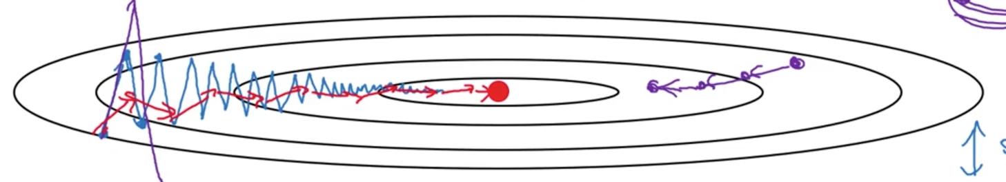
- Speed up for gradient descent:
- Gradient descent with momentum:
- Exponentially weighted averages: Bias in initial can be corrected phase by using bias correction.
- Momentum gradient decent is the method that gradient decent with exponentially weighted averages. The gradient oscillation in original gradient descent would be averaged. So the speed of that is faster than common gradient descent.
- In practice, people don't use bias correction (Vdw/1-beta),because after 10 iteration, the moving average would warmed up and no longer the bias estimate.
- The common choice of beta is 0.9.
- RMSprop (Root mean square prop):
- The vertical direction is represented by a and horizontal direction is w, RMSprop is aim to slow down variance of b and accelerate the speed of w.
- Gradient descent with momentum:
- Adam(adaptive moment estimation) optimization:
-
Momentum + RMSprop
-
Hyper-parameter
hyper-parameters heuristic value alpha tuning beta_monentum 0.9 beta_RMSprop 0.999 epsilon $e^{-8}$
-
- Mini-batch:
- Learning rate decay:
- There are many ways can adjust learning rate on line:
- Exponentially decay
- Stair decay
- Square root decay
- and so on...
- There are many ways can adjust learning rate on line:
- Fundamental concept and experience:
- Iteration: using data to update parameter one time that calls 1 iteration
- Epoch: Using through entire data once in many times of iterations called 1 epoch.
- Batch gradient descent: use all size of the data to update parameter. So here, 1 iteration equals 1 epoch. The parameters would be updated by k iterations (also k epochs)
- Stochastic gradient descent: use 1 of data to update parameters once. So here, iteration would be m (size of data), and the parameters would be updated by m*k times.
- Mini-batch: use a small batch of data to update parameter. So here, iteration would be m/mini-batch, and the parameter would be updated by k*m/mini-batch.
- Improve optimization:
- Try better random initialization for weights
- Use mini-batch
- Use Adam-descent
- Relatively low memory requirements (though higher than gradient descent and gradient descent with momentum)
- Usually works well even with little tuning of hyper-parameters (except
$\alpha$ )
- Tuning learning rate.

- Hyper-parameter tuning
- Hyper-parameter:
- Learning rate
$\alpha$ ***** - Momentum
$\beta$ - Adam:
$\beta_{1}$ ,$\beta_{2}$ ,$\epsilon$ - Number of layers
- number of hidden units
- Learning rate decay
- Learning rate
- Logarithm skill
- Hyper-parameter:
- Batch normalization
- Normalizing activation:
- Data normalization can make contour much rounder.
- Normalize the value of not a but z.
- It can make the training speed much faster.
-
$z_{norm}=(z_{old} - \mu)/\sigma$ ,$z_{new} = \alpha*z_{norm}+\beta$ .Here, parameter alpha and beta are controlling the distribution of z for each different activation unit.
-
$\beta$ and$\alpha$ can be learned as same as w and b. - Using batch normalization, the parameter of b would be helpless. because all the bias item would be eliminated by mean subtraction.
- Activation normalizing can keep the distribution stable and avoid the covariate shift brought from value change in previous layer.
- Practically, in test, for single test data, the mean and variance for each layer is computed from training mini-batch by exponentially weighted average.
- Normalizing activation:
- multi-class classification
- Softmax activation and loss is
$-\Sigma y_{i}log \hat{y_{i}}$
- Softmax activation and loss is
- Frameworks:
- Ease of programing
- Running speed
- Open source
- Assignment notes:
- The two main object classes in tensorflow are Tensors and Operators.
- When you code in tensorflow you have to take the following steps:
- Create a graph containing Tensors (Variables, Placeholders ...) and Operations (tf.matmul, tf.add, ...)
- Create a session
- Initialize the session
- Run the session to execute the graph
- You can execute the graph multiple times as you've seen in model()
- The back-propagation and optimization is automatically done when running the session on the "optimizer" object.
-
Motivating to ML strategy
data model regularization optimization more data bigger network dropout Longer GD more diverse train set small network L2... Adam more hidden units activation function -
Chain of assumption in ML
- Fit on training set --> dev set --> test set --> real world
- Experienced persons always know how to improve the model when they suffer form poor results in different occasions.
- For orthogonalization, not to use early stopping.
-
Set up training/dev/test set
- it is important to choose dev and test from same distribution which must be taken randomly from all the data.
-
Bayes optimal error: best possible error
-
In some applications such as image recognition, human error can be regarded as Bayes optimal error approximately. In one hand, if the training set is relatively far from it, it means the model is still under-fitting.In another hand, if the training error is close to the human error, alter to decrease dev error but not training error.
diff of train&human > diff of train&dev > bias deduction variance deduction high bias high variance under-fitting over-fitting change hyper-para regularization enlarge model reduce model try training longer add training set
- Error analysis
- Deep learning algorithm are quite robust to random error in the training set but not robust to the systematic error.
- Metric of fixing the miss-label in dev/test set is the percent of miss-labeled data in all the dev/test set.
- Apply same method to process dev and set to make them have same distribution.
- Consider examining examples your algorithm got right as well as the ones it got wrong.
- Perhaps, the training set and dev/test set come slightly from different distribution.
- Mismatched training and dev/test set
- Training set and dev/test set are on the different distribution:
- Don't mix and shuffle the training set and dev/test set. Just keep the original distribution of training set. But put half of dev/test set into training set, and the left half part of dev/test set would be in another same distribution. DL algorithm is strong to processing the training set with different kinds of distribution over the long term.
- How to choose to parts of dataset to lean?
- If the training set and dev set come from different distribution, we can't say high variance/bias we have got any longer.
- Make a small part of training-dev set, then observer the error different on training set and training-dev set.
- The error different between training-dev and dev set is big, it means data mismatch problem.
- DL algorithm is easy to over-fit on the subset of all the data.
- Training set and dev/test set are on the different distribution:
- Learning from multiple tasks:
- Transfer learning:
- By means of structure and parameters of the other model, if you have large size of training data for the new task, you can retrain all the parameters initializing with previous parameters. If the training set of new task is small, just retrain the last layer.
- Two concepts:
- Pre-training: the parameters from previous model.
- Fine-tuning: the parameters retrain from pre-training.
- When transfer learning makes sense.
- Task A and B have the same input x.
- You have a lot more data for task A than task B.
- Low level features from A could be helpful for learning B.
- Multiple tasks learning:
- When multi-task learning make sense:
- Training on a set of tasks that could benefit from having shared lower-level features.
- Amount of data you have for each task is quite similar.
- Can train a big enough neural network to do well on all the tasks.
- When multi-task learning make sense:
- Transfer learning:
- End-to-end learning:
- The training models are chosen based on size of training set.
- End-to-end methods can work well on large data set.
- Pros and cons:
- Pros:
- Let the data speak
- less hand-designing of components needed
- Cons:
- May need large amount of data
- Excludes potentially useful hand-designed components.
- Pros:
(latex math viewer: https://chrome.google.com/webstore/detail/github-with-mathjax/ioemnmodlmafdkllaclgeombjnmnbima/related)